
In July, Microsoft announced the general availability of Power BI 2.0, the official replacement for Power BI for Office 365 (Power BI 1.0). Since then, much ado has been made about the upgraded service and its extensive line of reporting and analytical capabilities.
Power BI delivers self-service business intelligence (BI) to knowledge workers, business analysts, and anyone else who needs to gain quick insight into data. With Power BI, you can create reports that contain a variety of rich visualizations, post those visualizations to your dashboard, share the information with other users, and access the dashboard and reports from your mobile devices.
Your Power BI visualizations can be based on data from a wide range of sources. For example, you can retrieve data from services such as Google Analytics, GitHub, Zendesk, or Visual Studio online, or you can pull data from local files or OneDrive. Power BI also supports several database options, including Azure SQL Database, Azure SQL Data Warehouse, a tabular instance of SQL Server Analysis Services (SSAS), and Spark on Azure HDInsight, as you can see in the following figure.
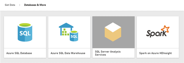
The figure shows the Power BI page you navigate to in order to connect to one of the database source types. You start by clicking the source type you want to use and then following the online prompts to provide the necessary information and credentials.
What’s interesting about all this, however, is not which database source types are included or how you set them up, but rather what source type is missing: SQL Server. Power BI does not provide a connector for an on-premises instance of SQL Server. For that, you must turn to Power BI Desktop.
Introducing Power BI Desktop
Power BI Desktop provides an integrated environment for retrieving and transforming data in order to define datasets that you can use to create reports containing different types of visualizations. After you’ve created your datasets and reports, you can publish them to the Power BI website, where you can work with them or share them as you would those created through the web tools.
Although similar to the Power BI service in many ways, Power BI Desktop provides a more robust environment for transforming data, in addition to being able to retrieve data from a wider range of sources, including SQL Server.
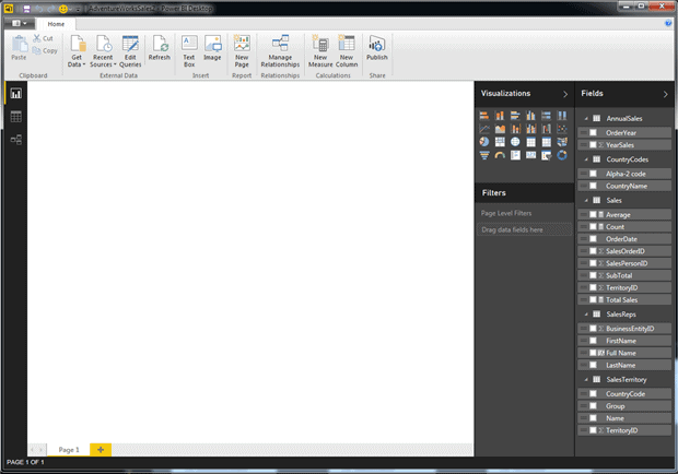
To get started with Power BI Desktop, you first need only download the program from the Microsoft Download Center and install it as you would any other desktop application. When you start it up, you’re presented with the user interface (UI) shown in the following figure.
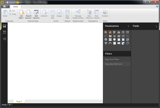
We’ll get more into many of the specifics of the UI as we work through the article. For now, the important feature to note is the left toolbar, which contains three options for accessing the views that define the report-creation workflow.
- Report view: Create reports that contain visualizations based on the transformed datasets. This is the default view when you open Power BI Desktop.
- Data view: Manage the datasets you created from the data you retrieved from the target sources. You can create data sets without this view being active.
- Relationships view: Define relationships between the datasets.
Another important component of the report-creation workflow is Query Editor, which opens in a window separate from the main UI. This is where you transform your datasets.
The rest of the article demonstrates how you can use Power BI Desktop to retrieve and transform data from SQL Server. I created the examples based on data from the AdventureWorks2014 database, which in my case, is on a local instance of SQL Server 2014.
Retrieving data from SQL Server
The place to start, of course, is to get the data we need. To initiate a connection to SQL Server, click the Get Data button on the Home ribbon, and then click SQL Server. If you want to see all available data sources, you can instead click More to open the Get Data dialog box (shown in the following figure). From there, you can navigate to the SQL Server option.
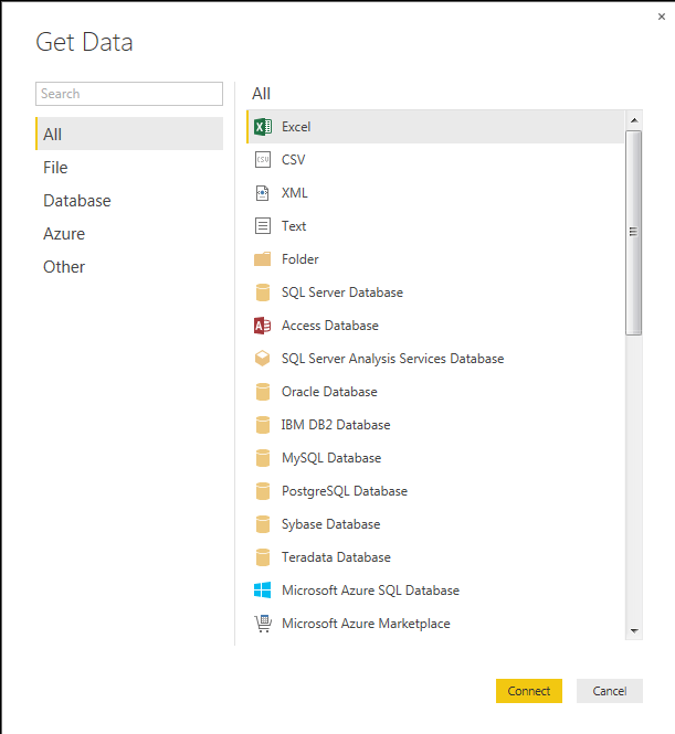
Whichever approach you take, you’ll be prompted to provide connection information, including the SQL Server instance and, optionally, the database name. You can also specify a T-SQL query at this time, if you want to be more precise in defining the data you initially return.
After you’ve connected to the SQL Server instance, the Navigator dialog box appears, where you can select the tables and views you want to import into Power BI Desktop, as shown in the following figure.
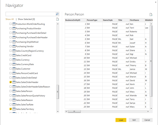
For our demo, we’ll pull the following three tables into Power BI Desktop:
- Person.Person
- Sales.SalesOrderHeader
- Sales.SalesTerritory
Notice at the bottom of the Navigator dialog box you have options for either loading the data or editing the data. If you click Load, you will load the data as is, and the tables will be added as datasets, which you can view in Data view. From there, you can launch Query Editor to transform the data or start using the data to create visualizations. Or you can instead click the Edit button to launch right into Query Editor, which is what we’ll do here.
Transforming data in Query Editor
Transforming the data is where all the fun begins. In Query Editor, you apply a series of steps to each data set in order to transform the data. Query Editor records each transformation in the Applied Steps box at the bottom of the Query Settings pane. The following figure shows the Person dataset, with two steps applied.
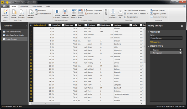
By default, a dataset starts with the steps Source and Navigation, which define the initial connection and data retrieval. At this point, the data is just as we imported it from the source database.
Our goal for the Person.Person table is to create a dataset that includes only the names and IDs of the Adventure Works sales reps. To define the dataset, we can start by using the PersonType column to filter out all rows except those with a value of SP. To apply the filter, click the arrow at the top of the column and, in the pop-up dialog box, clear all checkboxes except the SP option, as shown in the following figure.
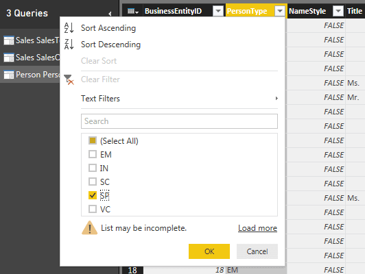
After you click OK, Query Editor removes all but the sales rep rows and adds a step named Filtered Rows to the Applied Steps box.
You can now continue to the next step, which is to remove all but the BusinessEntityID, FirstName, and LastName columns. To remove the other columns, click the header of the first column, press and hold the Control key, and click the other column headers. After you’ve selected all the columns to be deleted, right-click the header of one of the selected columns, and then click Remove Columns. Query Editor will remove the columns and add the Removed Columns step to the Applied Steps box.
The only transformation left is to sort the rows, based on the LastName value. To do so, once again click the arrow at the top of the column and click Sort Ascending. This sorts the rows and adds the Sorted Rows step to the Applied Steps box. You should be left with a dataset similar to what’s shown in the following figure.
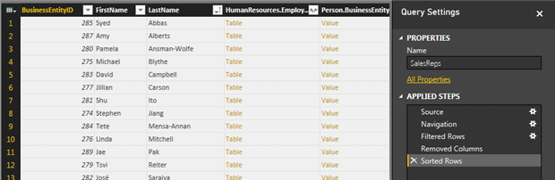
There are a couple items worth noting in the figure. First, you have a set of columns in your dataset that contain oddly colored values called Table and Value. Query Editor provides this information to point you to data related in other tables in the source data. However, this information does not show up in your final dataset.
You might have also noticed that I renamed the dataset to SalesReps, to make it more suitable to the type of data. In addition, we now have six steps in the Applied Steps box. Power BI Desktop retains these steps so we can return to the query at any time to view how the data was transformed as well as modify those transformations if needed. We can even move steps up or down or remove them altogether. Be careful, however, when you start changing or moving steps around because there can be dependencies between steps and you could end up with unexpected results.
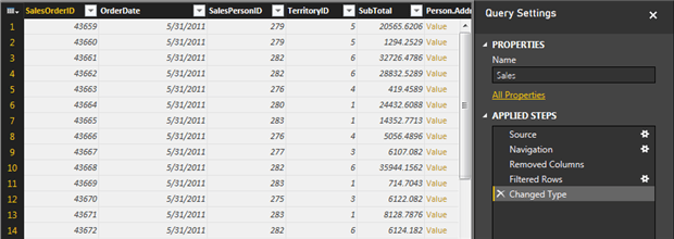
I won’t walk you through each step for transforming the other two datasets, but I’ll provide you with an overview so you can do it on your own. For the SalesOrderHeader table, change the name to Sales and apply the following transformations:
- Remove all columns except SalesOrderID, OrderDate, SalesPersonID, TerritoryID, and Subtotal.
- Filter out all rows with a SalesPersonID value of NULL.
- Change the data type of the OrderDate column to Date. To change the type, select the column and then, on the Transform ribbon, click Data Type and then click Date.
After you apply these transformations, you should end up with a dataset that looks similar to the one shown in the following figure.
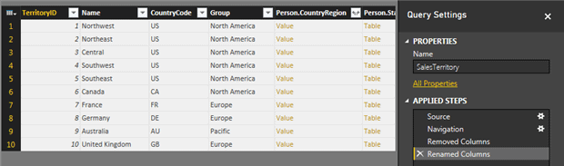
For the SalesTerritory table, shorten the name to exclude the schema and apply the following transformations:
- Remove all columns except TerritoryID, Name, CountryRegionCode, and Group.
- Rename the CountryRegionCode column to the CountryCode column.
Your final table should look something like what’s in the following figure.
That’s all there is to applying basic transformations to a dataset. Overall, Power BI Desktop makes this an intuitive and painless process. These might not be particularly complex transformations, but for some users, they will be plenty.
Query Editor includes lots of other types of transformations for performing such tasks as removing duplicates, splitting columns, merging queries, replacing values, pivoting data, or applying mathematical expressions. You can even access the DAX code underlying the dataset, as shown in the following figure, as well as access the DAX expressions used to transform the data.
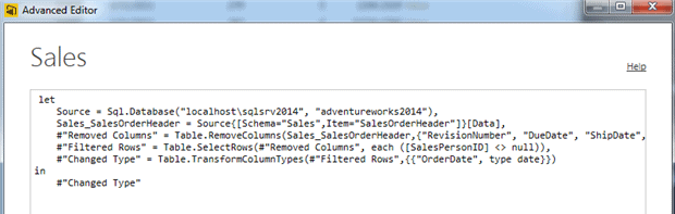
For now, working with these expressions, like other advanced features, is beyond the scope of this article (but will perhaps get covered in a subsequent article or two). For now, I encourage you to play around with the transformations and get a sense of what you can do in Query Editor. In the meantime, let’s look at a couple other steps we can take right now.
Grouping data in Query Editor
Power BI Desktop lets us group data just like we can in SQL Server. For example, suppose we want to include a visualization in our report that aggregates sales data across years. One approach we can take is to duplicate the Sales dataset and use the copy to create a separate, aggregated dataset.
To duplicate the Sales dataset in Query Editor, right-click the dataset in the left pane, and then click Duplicate. Change the name of the new dataset to AnnualSales, and then remove all but the OrderDate and SubTotal columns.
The next step is to extract the years from the values in the OrderDate column. To do so, select the column, and then, on the Transform ribbon, click Date, point to Year, and then click Year.
The next thing we need to do is to change the data type of the OrderDate column to text so our visualizations don’t treat them as numbers and try to aggregate them. To change the type, select the column and then, on the Transform ribbon, click Data Type and then click Text.
We are now ready to group the data. To do so, click the Group By button on the Transform ribbon. This launches the Group By dialog box, shown in the following figure.
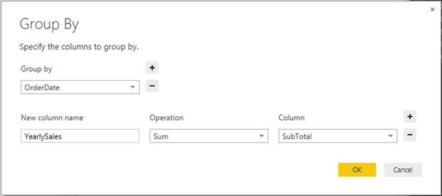
The figure shows how you should configure the settings to aggregate the SubTotal values based on the OrderDate column. We will end up with a column named YearlySales that shows the total amount of sales for each year.
Next, change the name of the OrderDate column to OrderYear by right-clicking the current column name and clicking Rename. You should end up with a dataset that looks similar to the one in the following figure.
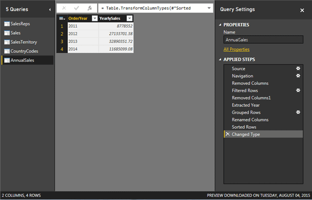
That’s all there is to grouping data. You might have noticed that the Applied Steps box includes all the original transformations from the Sales dataset. You can play with these if you like, or leave things just as they are. You could have also re-imported the table and grouped the data that way.
Retrieving data from the Web
Before we finish up with Query Editor, let’s add one more dataset. Suppose we want to create a visualization or two based on the CountryCode values in the SalesTerritory dataset, but want to display the actual country name. One approach we can take is to pull those names from someplace off the web and add it to our datasets.
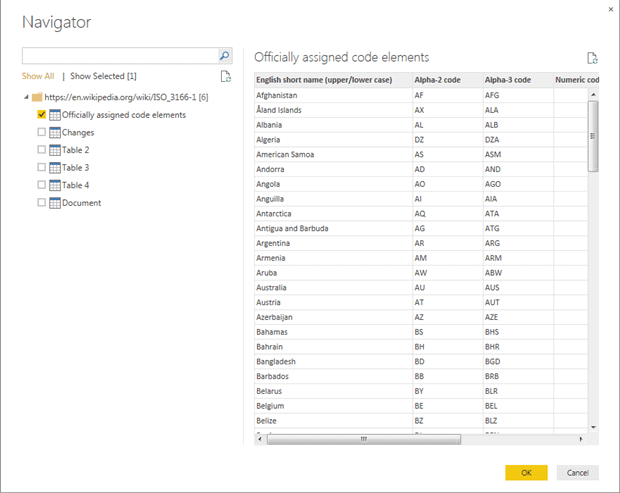
It turns out the Wikipedia has exactly what we need. Start by clicking the New Source button on the Home ribbon and then navigating to the Web connector type. (It’s part of the Other category.) When you click Web, the From Web dialog box appears, where you enter the following URL: https://en.wikipedia.org/wiki/ISO_3166-1.
When the Navigator dialog box appears, you’re presented with a list of tables available on that webpage, as shown in the following figure. Select Officially assigned code elements, and then click OK.
The new dataset opens in Query Editor. First, change the dataset name to CountryCodes and then apply the following transformations:
- Remove all but the English short name (upper/lower case) column and the Alpha-2 code column.
- Change the name of the English short name (upper/lower case) column to CountryName. You can also change the name of the Alpha-2 code column if you want, but I chose to leave it as it is for now.
You should end up with a dataset that looks similar to the one shown in the following figure:
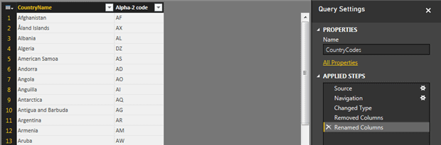
Notice that a Changed Type transformation has been added to the Applied Steps box. When Power BI Desktop imported the data from Wikipedia, it updated the column types to conform to the Power BI Desktop environment.
That’s all we need to do in Query Editor for now. Close Query Editor and return to the main Power BI Desktop window. To get out of Query Editor, click the Close & Load button on the Home ribbon. The datasets will now be available for viewing in Data view.
Adding a calculated column to a table
In Data view, you can review your datasets, using the Fields pane at the right to navigate through the datasets and their columns. You can also perform a few transformations, such as adding calculated columns or measures. Be aware, however, that elements you change in Data view are not reflected within the saved queries that you access through Query Editor.
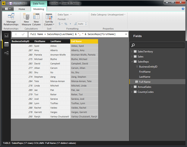
That said, let’s look at how to add a calculated column in Data view. Suppose we want to add a column to the SalesReps dataset that concatenates the first and last names, with the last name first. We’ll call the column Full Name. Start by clicking the New Column button on the Home or Modeling ribbon. This will add a blank column named Column and open a DAX formula bar at the top of the main window. To concatenate the two values, enter the following expression in the formula bar, replacing the current values:
Full Name = SalesReps[LastName] & “, ” & SalesReps[FirstName]
Next, click the checkmark to the left of the formula. This will verify that the DAX expression, update the new column, and populate it with the correct data, as shown in the following figure.
That’s all you need to do to add a calculated column. You can, of course, define far more complex DAX expressions than what we did here, but this should give you a sense of what you need to do and how easy it really is.
Adding measures to a table
It’s just as easy to add a measure to a dataset. A measure lets you aggregate data across different and changing dimensions. The aggregation can be based on one or more columns and applied to your visualizations to provide summarized views of the data.
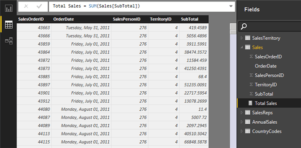
For our example, we’re going to add three measures to the Sales dataset. To create a measure, click the New Measure button on the Home or Modeling ribbon and then define the DAX formula. The first measure calculates the sum of the SubTotal values. Name the measure Total Sales and add the following DAX expression to the formula bar:
|
1 |
Total Sales = SUM(Sales[SubTotal]) |
The next measure, named Average, uses the following expression to determine the average number of sales:
|
1 |
Average = AVERAGE(Sales[SubTotal]) |
Finally, we’ll add a measure that counts the number of sales, which we’ll name Count. Use the following expression for this measure:
|
1 |
Count = COUNT(Sales[SalesOrderID]) |
After you’ve added the three measures, your Sales dataset should now look similar to the following figure.
Just like calculated columns, the DAX expressions you use to create measures can be far more complex than the ones we’ve added here. The more familiar you are with DAX, the more varied the type of measures you can create.
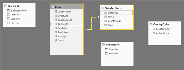
Managing relationships between data
Before you start creating your visualizations, you need to take one more step: define the relationships between our datasets. When you first set up your datasets, Power BI Desktop attempts to identify relationships that are already apparent. For example, if you go to the Relationships view, you should see all your datasets, with a relationship defined between the Sales and SalesTerritory datasets, based on the TerritoryID column in each dataset, as shown in the following figure.
You can view details about the relationship by clicking the Manage Relationships button on the Home ribbon. When the Manage Relationships dialog box appears, select the relationship if not selected, and then click Edit. The Edit Relationship box appears, providing details about the relationship, as shown in the following figure.
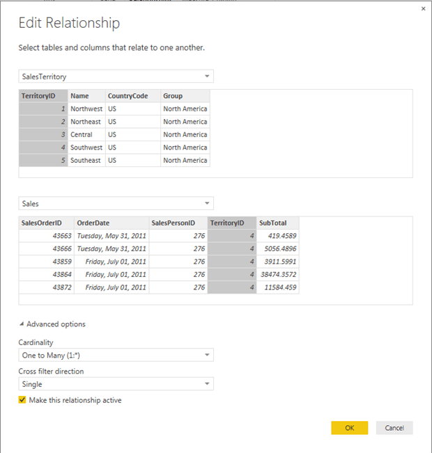
As you can see, the TerritoryID column in SalesTerritory is related to the TerritoryID column in Sales, defined as a one-to-many relationship between the two. If necessary, you can edit the relationship, although for one as straightforward as this one, it likely will not be needed.
If you return to the Manage Relationships dialog box, you’ll also find the AutoDetect button, which allows you to find other potential relationships. This feature will sometimes detect relationships that were not detected initially or find relationships after datasets have changed or new ones added.
If after all this undetected relationships still exist, you can manually define them by clicking Add in the Manage Relationships dialog box. When the Create Relationship dialog box appears, you can select the tables and columns on which to base the relationship. For example, we can define a relationship between the BusinessEntityID column in the SalesReps dataset and the SalesPersonID column in the Sales dataset, as shown in the following figure.
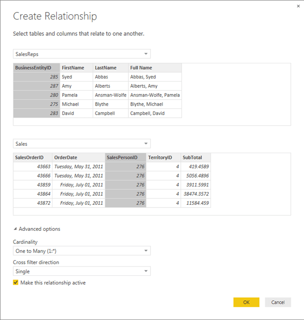
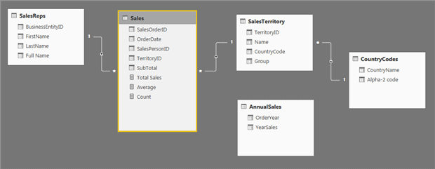
In this case, we’re defining a one-to-many relationship, from SalesReps to Sales. A relationship should also exist between the TerritoryID column in the SalesTerritory dataset and the Alpha-2 code column in the CountryCodes dataset (one-to-many from CountryCodes to SalesTerritory). The following figure shows the Relationships view with all the necessary relationships defined.
Having clearly defined relationships lets you use data from different datasets in a single visualization. Once you’ve defined your relationships, you’re ready to start building your reports. Note that you don’t have to have all your datasets and relationships completely defined before you start adding visualizations. You can always go back and tweak things. However, making changes after the fact can sometimes impact your visualizations in strange ways. But as you’ll see, creating visualizations so easy that having to redo a little work is no big deal.
Building reports
The report building capabilities in Power BI are fairly extensive and could easily justify an article or two of their own, but we can at least look at a few of them to help you get started.
When you first go to Report view, you’re provided with an empty slate (the report designer), as shown in the following figure. Here you can add visualizations, using the datasets you defined earlier, which are displayed in the Fields pane to the right. Just to the left of that pane is the Visualizations pane, which gives you the tools you need to add and configure your visualizations.
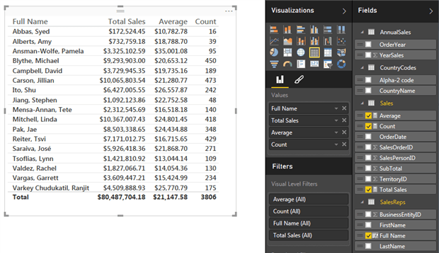
Let’s start by adding a simple table to our report that shows the full name of each sales rep, along with their sales figures (totals, averages, and number of sales). First, in the Fields pane, click the Full Name column in the SalesReps dataset. This will add the initial table to the report, with a column showing the full names. (The Table visualization is the default visualization type.)
Next, we add the measures we created in the Sales dataset, starting with Total Sales, then Average, and finally Count. Once again, you need only select the checkboxes associated with the three measures. Just be sure to check them in the order specified, or in the order you want them displayed in the visualization.
That’s all you need to do to create a Table visualization. The figure below shows what the table looks like and the fields selected to create it. You can resize or move the table, add or remove columns, or create filters on the individual columns.
If you want to display the data in a different visualization, simply click one of the visualization buttons in the top section of the Visualizations pane. In fact, try out a number of the visualizations. This can be a good way to get a feel of how the different visualizations work and what type of data works well in different situations.
Now let’s add a Donut Chart visualization to the report (the bottom right visualization button). To add the visualization, first make sure the table is not selected, and then click the Donut Chart button. A gray version of the chart is added to the report. Next, select the CountryName column in the CountryCodes dataset, and then select the Average measure in the Sales dataset. You should now have a visualization that looks like the one in the following figure. 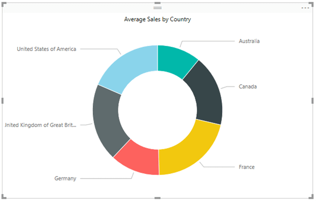
As with the table (or any visualization), you can resize and move it as necessary. The fun part of these types of visualizations, when used in conjunction with a table, is that you can select a section of the chart, such as France, and the data in the table will be updated to display sales amounts specific to that country
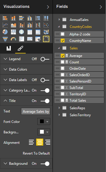
You can also modify the appearance of the visualizations. The degree to which you can make changes depends on the visualization type. To modify format settings, go to the Format tab in the Visualizations pane by clicking the Format button just below the list of visualization buttons. (It looks like a paintbrush.) On the Format tab for the Donut Chart visualization, you can change settings related to such elements as the data and category labels or data colors, as shown in the figure to the right.
For this example, I changed the title to read “Average Sales by County,” set the font color to black, and centered the label, but you can change the formatting however you like. Experiment with the options available to the various visualizations to see what you like. Whenever you make a change here, it is reflected immediately in the visualization.
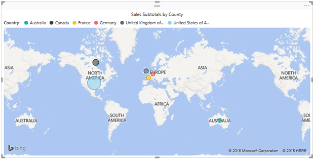
Now let’s add a Map visualization to the report. Once again, make sure that no visualization is selected, and then click the Map button in the Visualizations pane. For the Map visualization, select the CountryCode column from the SalesTerritory dataset, the Total Sales measure from the Sales dataset, and the CountryName column from the CountryCodes dataset. You can then configure the title or apply any other formatting that’s available to the visualization. When you’re finished, your visualization should look similar to the one shown in the following figure.
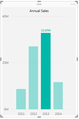
Finally, let’s add a Line and Clustered Column Chart visualization. For this, you need include only the OrderYear column and YearlySales measure from the AnnualSales dataset, giving you a visualization that looks similar to the one shown in the following figure. Again, you can format the visualization however you like, based on the formatting options available to that visualization.
When you’re finished, you should have a report that contains the same elements as those shown in the following figure. Be sure to save your Power BI Desktop file often to preserve all your fine work. When naming the file, keep in mind that this will be the name used if you publish the report and datasets to the Power BI site.
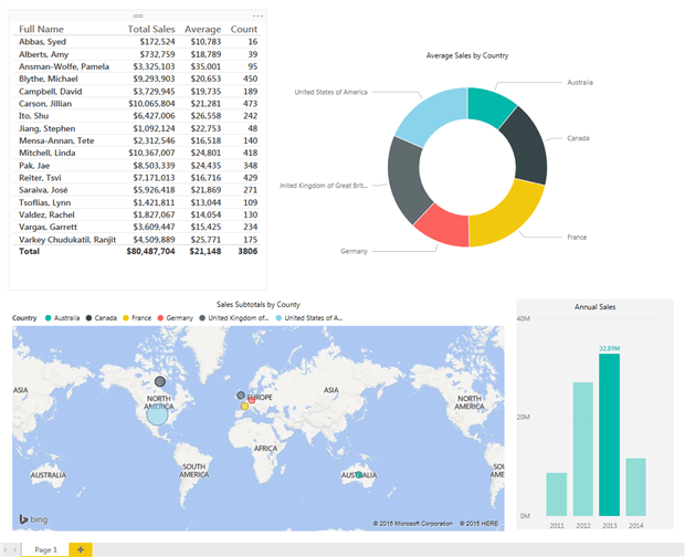
As you can see, adding visualizations to a report is relatively painless, once you have your datasets in place. And you can change the visualizations, resize and move them around, or add more pages for additional visualizations. You can also add text boxes or images.
Publishing reports to Power Bi
Once you’ve set up your reports and datasets the way you want them, you can publish them to the Power BI site. To do so, click the Publish button on the Home ribbon. If you’re already signed into Power BI, that’s all you need to do. Otherwise, you will also need to provide your Power BI credentials.
On the Power BI site, your report will be added to the Reports section in the left pane, and your dataset will appear in the Datasets section. Each one will be named whatever you named your Power BI Desktop file. From there, you can work with the reports and datasets just like you can with those created on the Power BI site.
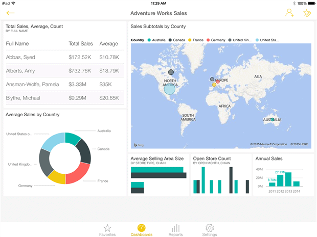
Another task you can perform in the BI site is to pin your report’s visualizations to a dashboard. For example, suppose you’ve created a dashboard named Adventure Works Sales and you want to add our four visualizations to the report. To do so, simply click the Pin Visual icon at the top right of the visualization and it will be added to the dashboard, as shown in the following figure.
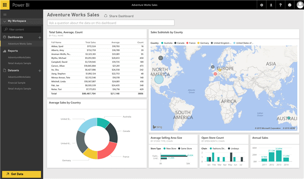
When working with visualizations on a dashboard, you’re limited to containers that are of a fixed size, but you can move the visualizations around and size them to fit the containers. As you can see in the figure, I’ve used three different sized containers. Notice too that I added a couple visualizations from another report (a sample available to Power BI).
There’s more you can do in Power BI, of course, but that will have to wait for a different article. In the meantime, another fun feature in Power BI is the ability to access your Power BI reports and dashboards from a mobile device. For example, the following figure shows the dashboard as it looks on an iPad.
Like the reports in Power BI Desktop, you can interact with the visualizations. For example, if you touch the Donut Chart visualization, it pops out and lets you spin the circle to so you can view the data about a specific country, as shown in the following figure. 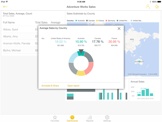
You can perform a number of other tasks as well, such as view the reports or specify certain visualizations as favorites. Microsoft provides apps for iOS, Android, and Windows mobile devices. The best part about the Power BI platform, which includes the mobile apps, Power BI Desktop, and Power BI site, is that a basic account is free and you have full access to everything we’ve covered here. And if you opt for a Power BI Pro account at $9.99 per month, you have more options for consuming data and integrating your reports.
Plenty more where they came from
We’ve only skimmed the surface of the many things you can do with Power BI and Power BI Desktop, especially when it comes to transforming data. But what we covered should give you a sense of the basic workflow and how easy it is to get started.
The ability to use Power BI Desktop to connect to an on-premises instance of SQL Server makes the platform all the more attractive. You can create SQL Server datasets and reports locally, publish them to the Power BI site, and share the site with other users, who can then create reports of their own based on the data. Power BI and Power BI Desktop also provide other options for sharing. Indeed, as a tool for providing users with self-service BI, the Power BI platform has much to offer.
This document contains proprietary information and is protected by copyright law.
Copyright © 2026 Red Gate Software Limited. All rights reserved


Load comments