
The series so far:
- SQL Server R Services: The Basics
- SQL Server R Services: Digging into the R Language
- SQL Server R Services: Working with ggplot2 Statistical Graphics
- SQL Server R Services: Working with Data Frames
- SQL Server R Services: Generating Sparklines and Other Types of Spark Graphs
- SQL Server R Services: Working with Multiple Data Sets
In the first article in this series, I introduced you to the concept of the data frame, a type of object in the R language for working with a set of related data, similar to a table variable in SQL Server. The second and third articles also touched upon data frames, but only in passing. In this article, we dig into the data frame in much more detail.
Data frames are an important concept in the R language and are integral to understanding how to write R scripts when working with SQL Server R Services. In fact, much of the work you do within an R script is related to creating data frames, restructuring them, or transforming their data in some way. You can, of course, incorporate other object types, such as vectors or lists, but you must still rely heavily on the data frame structure.
For example, when you create an R script that leverages SQL Server data, you use the InputDataSet variable to import the data into the script. To return the script’s output to a calling application, you use the OutputDataSet variable. Both variables come as part of the R Services package and are defined with the data.frame type, an R class used to structure an object as a data frame.
Another way to look at this is that a typical R script in SQL Server starts with a data frame and ends with a data frame, with operations carried out in between. Even if you pass the data into a ggplot2 visualization—and don’t return the data to an application—you must get the data into a data frame.
Introducing the R data frame
The data frame is one of the most widely implemented data objects in R, providing table-like structures for manipulating and analyzing sets of data. Like a SQL Server table, a data frame is made up of rows and columns. The rows are sometimes referred to as observations, and the columns referred to as variables. In fact, you can think of a data frame as a collection of variables that have the same length (number of rows).
As already noted, R Services includes two important data frame variables: InputDataSet and OutputDataSet. You can write a simple R script that uses the InputDataSet variable to access SQL Server data, and use the OutputDataSet variable to return that data to a calling application, without doing anything in between, as shown in the following T-SQL script:
|
1 2 3 4 5 6 7 8 9 10 11 12 13 14 15 |
USE AdventureWorks2014; GO DECLARE @rscript NVARCHAR(MAX); SET @rscript = N' OutputDataSet <- InputDataSet'; DECLARE @sqlscript NVARCHAR(MAX); SET @sqlscript = N' SELECT h.Subtotal, t.Name AS Territories FROM Sales.SalesOrderHeader h INNER JOIN Sales.SalesTerritory t ON h.TerritoryID = t.TerritoryID;'; EXEC sp_execute_external_script @language = N'R', @script = @rscript, @input_data_1 = @sqlscript; GO |
The R script is about as basic as you can get in SQL Server. It assigns the data from the InputDataSet variable to the OutputDataSet variable, copying the data from one data frame object to another in order to return the data to the application that called the sp_execute_external_script stored procedure. (For information about the various T-SQL elements in the above example, refer to the previous articles in this series.)
Normally, a SQL Server R script would contain far more logic between the InputDataSet and OutputDataSet variables, transforming the data along with way. In fact, this example is so simple that we can achieve the same results by running the SELECT statement alone, without all the other T-SQL trappings, but I wanted to approach this topic one step at a time. To this end, let’s start by confirming the data type of the InputDataSet variable, which we can do by using the class function, as in the following SET statement:
|
1 2 3 |
SET @rscript = N' df_class <- class(InputDataSet) print(df_class)'; |
Note that in this example and the ones to follow, I show only the SET statement used to assign the R script to the @rscript variable. The other T-SQL elements are the same throughout all the examples, so I opted not to repeat them each time. Just know that you must run every T-SQL statement shown in the first example if trying out the other examples.
Returning now to the above example, all we’re doing here is specifying the InputDataSet variable as an argument to the class function and then assigning the results to the df_class variable. We then use the print function to return the df_class value. If we now run the T-SQL code, it will confirm that the InputDataSet variable uses the data.frame type.
Now let’s assign the InputDataSet variable to the sales variable and then retrieve the data type for the new variable:
|
1 2 3 |
SET @rscript = N' sales <- InputDataSet print(class(sales))'; |
Once again, the R script indicates that the variable uses the data.frame type. If we were to view the contents of the sales variable, we would see that it contains our SQL Server data.
Next, we’ll assign the sales variable to the OutputDataSet variable and use the class function to retrieve the data type for that variable:
|
1 2 3 4 |
SET @rscript = N' sales <- InputDataSet OutputDataSet <- sales print(class(OutputDataSet))'; |
This time the R script will return all rows in the data set, followed by a message that indicates the OutputDataSet variable uses the data.frame type. As the examples demonstrate, we start with a data frame and end with a data frame, bringing the SQL Server data along the way.
Creating a data frame
When developing R scripts in SQL Server, you’ll likely want to construct data frames to help with your analyses. The data frames might use data from the InputDataSet variable, data brought in through another source, or a combination of both. The R language supports a wide range of possibilities when it comes to mixing and matching data.
To demonstrate how to build a data frame, we’ll create one with two columns, defining one column at a time. Although each column in a data frame must be the same length, you can add columns made up of different types of data, whether lists, vectors, factors, numeric matrices, or other data frames.
We’ll start by defining the data frame’s first column, which is based on the values in the Territories column of our SQL Server data set:
|
1 2 3 4 |
SET @rscript = N' sales <- InputDataSet c1 <- levels(sales$Territories) print(c1)'; |
The levels function retrieves a list of distinct values from the Territories column in the sales data frame. When referencing the column, we must first specify the sales variable, followed by a dollar sign ($), and then the column name. We then assign the output of the levels function to the c1 variable, which gives us what we need to create the first column.
For this example, I’m also tagging on the print function so we can view the c1 content. The R script returns the following results:
|
1 2 3 4 |
STDOUT message(s) from external script: [1] "Australia" "Canada" "Central" "France" [5] "Germany" "Northeast" "Northwest" "Southeast" [9] "Southwest" "United Kingdom" |
In SQL Server, when we return data from an R script in this way, without using the OutputDataSet variable, we get the data in a format such as that shown above. This approach provides us with a quick way to confirm an object’s values as we’re building our data frame.
Now let’s define the second column. This time, we’ll use the tapply function to return the aggregated means of the Subtotal values, grouped by sales territory:
|
1 2 3 4 5 |
SET @rscript = N' sales <- InputDataSet c1 <- levels(sales$Territories) c2 <- round(tapply(sales$Subtotal, sales$Territories, mean)) print(c2)'; |
The tapply function takes three arguments. The first is the Subtotal column in the sales data set. This column contains the values that will be aggregated.
The second argument is the Territories column in the sales dataset. This argument determines the factors used in aggregating the data. In other words, the Territories column provides the basis for how the values in the Subtotal column will be grouped together and aggregated. The unique territory names also provide a mechanism for indexing the aggregated values.
The third argument determines how the data will be aggregated. Because we’ve specified the mean option, SQL Server will return the mean subtotal for each territory. Notice that we also use the round function to round the aggregated totals to integers.
We can then use the print function to return the values in the C2 column, which are shown in the following results:
|
1 2 3 4 5 |
STDOUT message(s) from external script: Australia Canada Central France Germany 1557 4022 20543 2714 1874 Northeast Northwest Southeast Southwest United Kingdom 19714 3501 16213 3886 2383 |
Although the results might be a bit tricky to read, they confirm that we have the data we need in the C2 column, with the territory names acting as an index for the Subtotal values. We can now create a data frame that uses the Subtotal values in conjunction with the Territories values in the C1 column. To do so, we use the data.frame function to join the columns into a data frame:
|
1 2 3 4 5 6 |
SET @rscript = N' sales <- InputDataSet c1 <- levels(sales$Territories) c2 <- round(tapply(sales$Subtotal, sales$Territories, mean)) sales2 <- data.frame(c1, c2) OutputDataSet <- sales2'; |
When we call the data.frame function, we pass in the c1 and c2 variables as arguments. We then save the function’s output to the sales2 variable, giving us a data frame that we can then assign to the OutputDataSet variable. When we run the R script, we get the results shown in the following figure.
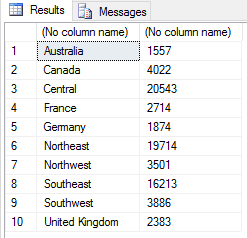
We can assign names to the outputted columns when calling the sp_execute_external_script stored procedure, but we don’t need to be concerned about that right now. However, if you want to add column names and are uncertain how to do that, refer to the first article in this series.
Retrieving data frame information
When working with data frames, we can retrieve information about them in order to verify data or troubleshoot a script. For example, we can retrieve a data frame’s length, dimensions, number of columns, and number of rows, as shown in the following example:
|
1 2 3 4 5 6 7 8 9 |
SET @rscript = N' sales <- InputDataSet c1 <- levels(sales$Territories) c2 <- round(tapply(sales$Subtotal, sales$Territories, mean)) sales2 <- data.frame(c1, c2) print(length(sales2)) print(dim(sales2)) print(ncol(sales2)) print(nrow(sales2))'; |
First, we use the length function to determine the object’s length, which for data frames, translates to the number of variables (columns). We then call the dim function to return the data frame’s dimensions, which gives us the number of rows and columns.
The R script then calls the ncol function to return the data frame’s number of columns (just like length), and the nrow function to return the number of rows. When we run the script, we get the following results:
|
1 2 3 4 5 |
STDOUT message(s) from external script: [1] 2 [1] 10 2 [1] 2 [1] 10 |
As you can see, the functions provide a simple way to return specific types of information. In addition to using them for verification and troubleshooting, we can also incorporate them within a script’s logic to control statement flow based on the returned values.
Another option we can use for getting information about a data frame is to call the summary function, passing in the data frame as an argument:
|
1 2 3 4 5 6 |
SET @rscript = N' sales <- InputDataSet c1 <- levels(sales$Territories) c2 <- round(tapply(sales$Subtotal, sales$Territories, mean)) sales2 <- data.frame(c1, c2) print(summary(sales2))'; |
The summary function returns specifics about each column in the data frame, as shown in the following results:
|
1 2 3 4 5 6 7 8 9 |
STDOUT message(s) from external script: c1 c2 Australia:1 Min. : 1557 Canada :1 1st Qu.: 2466 Central :1 Median : 3694 France :1 Mean : 7641 Germany :1 3rd Qu.:13165 Northeast:1 Max. :20543 (Other) :4 |
The information returned by the summary function varies depending upon the type of data in a column. For example, the c1 column includes unique character values, so the function simply lists several initial values, each followed by a 1, which indicates that there that there is only one instance of this value. The column summary then ends with a grouping of the remaining values (Other), followed by the number of those values, in this case, 4.
The c2 column includes only numeric values, so the summary function instead returns the minimum, median, mean, and maximum values, along with the first and second quartiles. The first quartile shows that about 25% of the values fall below 2466, and the third quartile shows that about 75% of the values fall below 13165.
We can also use the str function to return information about a data set, as shown in the following example:
|
1 2 3 4 5 6 |
SET @rscript = N' sales <- InputDataSet c1 <- levels(sales$Territories) c2 <- round(tapply(sales$Subtotal, sales$Territories, mean)) sales2 <- data.frame(c1, c2) print(str(sales2))'; |
The str function returns an object’s internal structure and provides an abbreviated list of its contents, as shown in the following results:
|
1 2 3 4 5 6 7 |
STDOUT message(s) from external script: 'data.frame': 10 obs. of 2 variables: $ c1: Factor w/ 10 levels "Australia","Canada",..: 1 2 3 4 5 6 7 8 9 10 $ c2: num [1:10(1d)] 1557 4022 20543 2714 1874 ... ..- attr(*, "dimnames")=List of 1 .. ..$ : chr "Australia" "Canada" "Central" "France" ... NULL |
The first line tells us that the object is indeed a data frame and that it contains 10 rows (observations) and 2 columns (variables). We then get details about each of the two columns. In this case, the results indicate that the c1 column is a factor variable containing a vector with 10 levels, and the c2 column is a numeric variable containing a vector with 10 elements. Each listing also includes a sample of the data. Plus, the c2 listing, which is made up of three lines, includes additional information about its index.
Manipulating data frame columns
In addition to being able to view information about a data frame, the R language lets you manipulate its rows and columns. For example, you can add columns, reorder them, or delete them. (We’ll get to rows in the next section.) Let’s start with adding a column. To do so, we simply define a new variable and then use the cbine function to add that variable to the primary data frame, as in the following script:
|
1 2 3 4 5 6 7 8 |
SET @rscript = N' sales <- InputDataSet c1 <- levels(sales$Territories) c2 <- round(tapply(sales$Subtotal, sales$Territories, mean)) sales2 <- data.frame(c1, c2) c3 <- c("AU", "CA", "US", "FR", "DE", "US", "US", "US", "US", "GB") sales3 <- cbind(sales2, c3) OutputDataSet <- sales3'; |
The first part of the script defines the initial data frame (sales2), as we’ve seen in preceding examples. Next, we define the c3 variable by creating a vector containing 10 values that coincide with the data frame’s existing rows and values. Notice that we must use the c function to concatenate the values before assigning them to the c3 variable.
In this example, we’re taking a very simple and manual approach to defining our column, but know that the R language lets us construct columns in a variety of ways, as well as import data from different source types, such as .csv files. In this way, we can create data frames that include a wide range of data from both SQL Server and other sources.
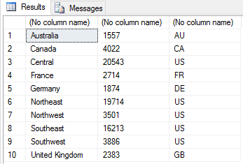
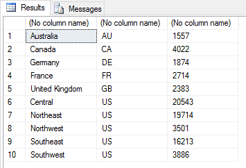
After defining the c3 variable, we use the cbine function to append the variable to the sales2 data frame. We then assign the function’s output to the sales3 variable. When calling the cbine function, we need only specify the sales2 data frame and c3 variable as arguments. From there, we assign the sales3 variable to the OutputDataSet variable, giving us the following results.
In some cases, we might want to rearrange the columns in the data frame. For example, we can move the c3 column to the second position by using the data frame’s indexing:
|
1 2 3 4 5 6 7 8 |
SET @rscript = N' sales <- InputDataSet c1 <- levels(sales$Territories) c2 <- round(tapply(sales$Subtotal, sales$Territories, mean)) c3 <- c("AU", "CA", "US", "FR", "DE", "US", "US", "US", "US", "GB") sales2 <- data.frame(c1, c2, c3) sales2 <- sales2[c(1,3,2)] OutputDataSet <- sales2'; |
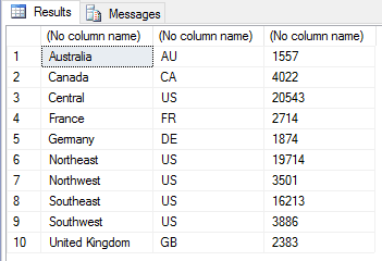
This time around, we’re creating the sales2 data frame as a single operation. We then call the data frame, followed by square brackets that specify the column order. In the R language, the brackets act as a subsetting function that lets us filter our datasets. We can create filter conditions based on rows, columns, or both. If we want to create a condition based on columns, but not rows, we include only a single argument, which in this case, is the new column order, based on their internally generated index numbers. Note, however, we must also use the c function to concatenate the list of indexes when reshuffling them in this way. We then reassign the changes back to the sales2 variable, giving us the results shown in the following figure.
Now suppose we want to delete the c3 column from the data frame. To do so, we simply set the value of that column to NULL, as shown in the following script:
|
1 2 3 4 5 6 7 8 |
SET @rscript = N' sales <- InputDataSet c1 <- levels(sales$Territories) c2 <- round(tapply(sales$Subtotal, sales$Territories, mean)) c3 <- c("AU", "CA", "US", "FR", "DE", "US", "US", "US", "US", "GB") sales2 <- data.frame(c1, c2, c3) sales2$c3 <- NULL OutputDataSet <- sales2'; |
When referencing the c3 column, we specify the sales2 data frame, followed by a dollar sign ($) and then the column name. From there, we need only assign NULL to the column reference. This will remove the c3 column from the data set and leave us with only the c1 and c2 columns.
Manipulating data frame rows
We can also add rows to a data frame or remove them. For example, to add a row to our sales2 data frame, we define a new data frame that contains two columns and one row, and then use the rbind function to insert the row into the original data frame:
|
1 2 3 4 5 6 7 8 9 |
SET @rscript = N' sales <- InputDataSet c1 <- levels(sales$Territories) c2 <- round(tapply(sales$Subtotal, sales$Territories, mean)) sales2 <- data.frame(c1, c2) names(sales2) <- c("Territories", "Sales") r1 <- data.frame(Territories="New Zealand", Sales=1048) sales2 <- rbind(sales2, r1) OutputDataSet <- sales2'; |
The first thing to note here is that, after creating the sales2 data frame, we name the data frame’s columns. This provides us with more intuitive names for referencing the columns in subsequent statements. We could have instead provided different names for the original c1 and c2 variables or stuck with the c1 and c2 names throughout the entire script, but I wanted to demonstrate the ability to modify a data frame’s column names.
When assigning new columns names, we use the names function, passing in sales2 as an argument. We then use the c function to concatenate the list of new column names and pass the results to the names function.
With our data frame names in place, we’re ready to create our new row. To do so, we call the data.frame function and pass in the new values as arguments, using the updated column names when delineating those values. We then assign the results to the r1 variable.
After defining the row, we use the rbind function to add the row to the sales2 data frame, passing in the original data frame and new variable as arguments. We then reassign the output to the sales2 variable, giving us the following results.
If we want to delete a row from a data set, we essentially filter it out, reassigning the results to the existing variable or assigning them to a new one. For example, we can use the sales2 variable to create an expression that includes the logic necessary to filter out the row with a Territories value of New Zealand, as shown in the following example:
|
1 2 3 4 5 6 7 8 9 10 |
SET @rscript = N' sales <- InputDataSet c1 <- levels(sales$Territories) c2 <- round(tapply(sales$Subtotal, sales$Territories, mean)) sales2 <- data.frame(c1, c2) names(sales2) <- c("Territories", "Sales") r1 <- data.frame(Territories="New Zealand", Sales=1048) sales2 <- rbind(sales2, r1) sales3 <- sales2[sales2$Territories != "New Zealand",] OutputDataSet <- sales3'; |
We define our expression within a set of brackets that follow the sales2 variable. The expression begins by referencing the column name, rather than index number. We then use the not equal (!=) comparison operator to compare the column value to the string New Zealand. The comma at the end of the expression indicates that we’re subsetting the data by rows, not columns. (If we omit the comma, the R engine will assume we’re indexing by columns). We then assign the results to the sales3 data frame. The script will now return all rows except the one for New Zealand.
We can achieve the same results by using the subset function, as shown in the following example:
|
1 2 3 4 5 6 7 8 9 10 |
SET @rscript = N' sales <- InputDataSet c1 <- levels(sales$Territories) c2 <- round(tapply(sales$Subtotal, sales$Territories, mean)) sales2 <- data.frame(c1, c2) names(sales2) <- c("Territories", "Sales") r1 <- data.frame(Territories="New Zealand", Sales=1048) sales2 <- rbind(sales2, r1) sales3 <- subset(sales2, Territories != "New Zealand") OutputDataSet <- sales3'; |
The subset function allows us to return a subset or rows, columns, or both. When filtering out rows, we must pass in two arguments when calling the function. The first is the name of the data frame, and the second is the expression that defines the logic used for creating the filter. In this case, the script returns a subset of data that includes all rows except those that contain a Territories value of New Zealand. Because we’ve already specified the data frame in the first argument, we do not need to include it in the second argument to qualify the column name.
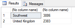
When subsetting row data, we can define a wide range of expressions. For example, the next script returns only those rows with a Sales value greater than 3000:
|
1 2 3 4 5 6 7 8 |
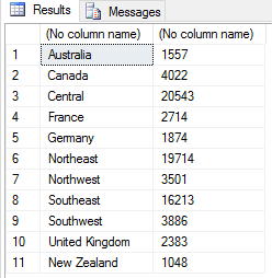
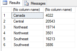
SET @rscript = N' sales <- InputDataSet c1 <- levels(sales$Territories) c2 <- round(tapply(sales$Subtotal, sales$Territories, mean)) sales2 <- data.frame(c1, c2) names(sales2) <- c("Territories", "Sales") sales2 <- subset(sales2, Sales > 3000) OutputDataSet <- sales2'; |
The R script returns the results shown in the following figure.
We can also create a compound expression when subsetting row data:
|
1 2 3 4 5 6 7 8 |
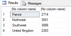
SET @rscript = N' sales <- InputDataSet c1 <- levels(sales$Territories) c2 <- round(tapply(sales$Subtotal, sales$Territories, mean)) sales2 <- data.frame(c1, c2) names(sales2) <- c("Territories", "Sales") sales2 <- subset(sales2, Sales > 2000 & Sales < 4000) OutputDataSet <- sales2'; |
This time we’re defining two conditions. The first specifies that Sales values must be greater than 2000, and the second specifies that Sales values must be less than 4000. The two conditions are connected by the and (&) logical operator, which means both conditions must evaluate to true, giving us the following results.
The ability to use conditional logic provides us with a wide range of options for subsetting rows. However, there might be times when we want to subset the columns, so let’s look at how to do that.
Creating Subsets of columns
The subset function also lets us filter out data based on specified columns. Again, we must pass in our data frame as the first argument, and then specify the columns we want to include in the results as the second argument:
|
1 2 3 4 5 6 7 8 |
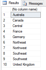
SET @rscript = N' sales <- InputDataSet c1 <- levels(sales$Territories) c2 <- round(tapply(sales$Subtotal, sales$Territories, mean)) sales2 <- data.frame(c1, c2) names(sales2) <- c("Territories", "Sales") sales2 <- subset(sales2, select="Territories") OutputDataSet <- sales2'; |
To ensure that we’re targeting columns, and not rows, we include the argument name (select) when specifying the columns we want to include. In this case, we’re specifying only the Territories column, giving us the following results.
We can achieve the same results by specifying the data frame variable and then, in brackets, providing the column name:
|
1 2 3 4 5 6 7 |
SET @rscript = N' sales <- InputDataSet c1 <- levels(sales$Territories) c2 <- round(tapply(sales$Subtotal, sales$Territories, mean)) sales2 <- data.frame(c1, c2) names(sales2) <- c("Territories", "Sales") OutputDataSet <- sales2["Territories"]'; |
Rather than using the column name, we can use the column’s assigned index number, which in this instance is 1:
|
1 2 3 4 5 6 7 |
SET @rscript = N' sales <- InputDataSet c1 <- levels(sales$Territories) c2 <- round(tapply(sales$Subtotal, sales$Territories, mean)) sales2 <- data.frame(c1, c2) names(sales2) <- c("Territories", "Sales") OutputDataSet <- sales2[1]'; |
It’s not uncommon in the R language to have multiple options for achieving the same results. In this case, we’re simply subsetting the data to filter out a column, but the same principle holds true if we want to filter out both rows and columns. Consider the following example, in which the subset function is used to return only those rows with a Sales value greater than 10000 and only the Territories column:
|
1 2 3 4 5 6 7 8 |
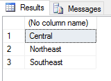
SET @rscript = N' sales <- InputDataSet c1 <- levels(sales$Territories) c2 <- round(tapply(sales$Subtotal, sales$Territories, mean)) sales2 <- data.frame(c1, c2) names(sales2) <- c("Territories", "Sales") sales2 <- subset(sales2, Sales>10000, select="Territories") OutputDataSet <- sales2'; |
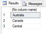
Again, when calling the subset function, we pass in the name of the data frame as the first argument. Next, we provide an expression to filter out row data, and finally we specify that only the Territories column be returned, giving us the results shown in the following figure.
We can also use indexing to return specific results, as we’ve seen in previous examples. Only this time, we must specify two elements within the brackets. The first is the rows to return, and the second is the columns to returns, as in the following example:
|
1 2 3 4 5 6 7 8 |
SET @rscript = N' sales <- InputDataSet c1 <- levels(sales$Territories) c2 <- round(tapply(sales$Subtotal, sales$Territories, mean)) sales2 <- data.frame(c1, c2) names(sales2) <- c("Territories", "Sales") sales3 <- data.frame(sales2[1:3, 1]) OutputDataSet <- sales3'; |
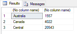
Notice that we’re using the data.frame function to format the filtered output as a data frame, passing in the sales2 data frame as an argument to the function. We’re also indexing the sales2 data frame to narrow down the results, specifying that only rows 1 through 3 be returned and only the first column (Territories) be returned. The following figure shows what our results look like this time around.
We can use a data frame’s indexing capabilities in any way necessary. For example, the next R script specifies that the rows 2 and 4 be returned, along with the first two columns:
|
1 2 3 4 5 6 7 8 |
SET @rscript = N' sales <- InputDataSet c1 <- levels(sales$Territories) c2 <- round(tapply(sales$Subtotal, sales$Territories, mean)) sales2 <- data.frame(c1, c2) names(sales2) <- c("Territories", "Sales") sales3 <- data.frame(sales2[c(2,4), 1:2]) OutputDataSet <- sales3'; |
When specifying the rows, we must use the c function to concatenate them because we are providing individual values, rather than a range. The script now returns the following results.
Not surprisingly, there is a great deal more we can do when it comes to subsetting a data frame. The better you understand how to filter data, the more effectively you can put together R scripts.
Making head or tail of a data frame
The R language provides a couple very handy functions for returning only the first or last few rows of a data frame. One of these is the head function, shown in the following example:
|
1 2 3 4 5 6 7 |
SET @rscript = N' sales <- InputDataSet c1 <- levels(sales$Territories) c2 <- round(tapply(sales$Subtotal, sales$Territories, mean)) sales2 <- data.frame(c1, c2) names(sales2) <- c("Territories", "Sales") OutputDataSet <- head(sales2, 3)'; |
The head function takes one or two arguments. The first argument is the target object, in this case, the sales2 data frame, and the second argument, which is optional, is the number of rows to return. Because we’ve specified 3, the script returns the following results.
If we had not specified the number of rows, the script would have returned six rows (or fewer rows, if the dataset had been smaller).
The R language also supports the tail function, which works just like the head function, except that it returns rows at the end of the data frame:
|
1 2 3 4 5 6 7 |
SET @rscript = N' sales <- InputDataSet c1 <- levels(sales$Territories) c2 <- round(tapply(sales$Subtotal, sales$Territories, mean)) sales2 <- data.frame(c1, c2) names(sales2) <- c("Territories", "Sales") OutputDataSet <- tail(sales2, 2)'; |
This time, we’ve specified that the last two rows be returned, giving us the following results:
As with the head function, the tail function returns up to six rows if no row amount is specified.
Turning things around in a data frame
The R language also provides the ability to sort a data frame, based on the values in one or more columns. For this, we use the order function:
|
1 2 3 4 5 6 7 8 |
SET @rscript = N' sales <- InputDataSet c1 <- levels(sales$Territories) c2 <- c("AU", "CA", "US", "FR", "DE", "US", "US", "US", "US", "GB") c3 <- round(tapply(sales$Subtotal, sales$Territories, mean)) sales2 <- data.frame(c1, c2, c3) names(sales2) <- c("Territories", "CountryCode", "Sales") OutputDataSet <- sales2[order(sales2$CountryCode, sales2$Territories),]'; |
When sorting a data frame, we first specify the data frame and then, within brackets, call the order function, passing in the column names as arguments. In this example, we’re sorting the data first by the CountryCode column and then by the Territories column, giving us the following results.
The R language also lets us pivot a data frame, turning rows into columns and columns into rows. For this, we use the t function (short for transpose), as shown in the following example:
|
1 2 3 4 5 6 7 8 9 |
SET @rscript = N' sales <- InputDataSet c1 <- levels(sales$Territories) c2 <- c("AU", "CA", "US", "FR", "DE", "US", "US", "US", "US", "GB") c3 <- round(tapply(sales$Subtotal, sales$Territories, mean)) sales2 <- data.frame(c1, c2, c3) names(sales2) <- c("Territories", "CountryCode", "Sales") sales2 <- data.frame(t(subset(sales2, Sales<3000))) OutputDataSet <- sales2'; |
Before pivoting the data frame, we use the subset function to filter out all rows except those with a Sales value greater than 3000. (I included this only to make the data easier to view once pivoted.) We then use the t function to pivot the subset, passing the function results in as an argument to the data.frame function. We then reassign the transposed data frame to the sales2 variable, giving us the results shown in the following figure.
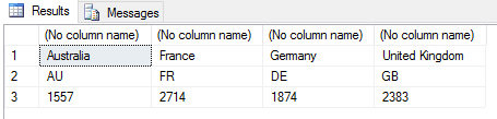
As you can see, we now have a column for each subsetted territory, rather than a row, with each column containing data relevant to its respective territory.
Updating data frame values
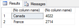
One other aspect of data frames worth looking at is how to update a specific value. To do so, we need only assign the new value to the specific column and row. For example, suppose we want to update the amount of France’s sales. To do so, we must assign the new value to the Sales column, filtering by the France territory, as shown in the following R script:
|
1 2 3 4 5 6 7 8 9 |
SET @rscript = N' sales <- InputDataSet c1 <- levels(sales$Territories) c2 <- c("AU", "CA", "US", "FR", "DE", "US", "US", "US", "US", "GB") c3 <- round(tapply(sales$Subtotal, sales$Territories, mean)) sales2 <- data.frame(c1, c2, c3) names(sales2) <- c("Territories", "CountryCode", "Sales") sales2$Sales[sales2$Territories=="France"] <- 2200 OutputDataSet <- sales2'; |
First, we call the Sales column and then, in brackets, specify that the Territories column value should equal France. Once we have constructed the basic elements, we need only assign the 2200 value to the Sales column. When we run the script, the R engine will update the value in the data frame and return the new results.
The ubiquitous data frame
To say that there is much more we can do with data frames than what we covered here would be a gross understatement. As a key structure of the R language, the data frame supports a wide range of options for manipulating and analyzing data.
There are, of course, many other important objects in R, and you will have to understand those as well to use R effectively in SQL Server. But data frames are key to working with the R language within R Services. You should know how to create them, update them, get information about them, and retrieve subsets of data from them. Only then will you be able to effectively use R services to manipulate and analyze data within the SQL Server environment.
This document contains proprietary information and is protected by copyright law.
Copyright © 2026 Red Gate Software Limited. All rights reserved


Load comments