
The series so far:
- SQL Server Machine Learning Services – Part 1: Python Basics
- SQL Server Machine Learning Services – Part 2: Python Data Frames
- SQL Server Machine Learning Services – Part 3: Plotting Data with Python
- SQL Server Machine Learning Services – Part 4: Finding Data Anomalies with Python
- SQL Server Machine Learning Services – Part 5: Generating multiple plots in Python
- SQL Server Machine Learning Services – Part 6: Merging Data Frames in Python
If you’ve spent any time with the R language in SQL Server R Services or Machine Learning Services (MLS), you’re no doubt aware of the important role that data frames can play in your scripts, whether working with data that comes from a SQL Server database or from another source. The same is true for Python. You use data frames when passing data sets into and out of a script as well as when manipulating and analyzing data within that script.
This article focuses on using data frames in Python. It is the second article in a series about MLS and Python. The first article introduced you briefly to data frames. This article continues that discussion, describing how to work with data frame objects and the data within those objects.
Data frames and the functions they support are available to MLS and Python through the pandas library. The library is available as a Python module that provides tools for analyzing and manipulating data, including the ability to generate data frame objects and work with data frame data. The pandas library is included by default in MLS, so the functions and data structures available to pandas are ready to use, without having to manually install pandas in the MLS library.
This article includes a number of examples that leverage the pandas library to demonstrate various data frame concepts, using data from the AdventureWorks2017 sample database. As you’ll recall from the first article, you can specify a T-SQL query when calling the sp_execute_external_script stored procedure and then incorporate the data returned by that query into your Python script. The examples that follow all use the same T-SQL query, allowing us to focus specifically on the Python scripts and data frame concepts.
Introducing the data frame
The pandas library supports a variety of data structures. The two most commonly used for analytics are Series and DataFrame. The Series data structure is an indexed, one-dimensional array whose values can be any Python data type, including strings, integers, floating point numbers, and other Python objects. The DataFrame data structure is an indexed, two-dimensional array that includes one or more columns, similar to an Excel spreadsheet or SQL Server table. All columns in a data frame are Series objects of the same length.
To better understand the Series and DataFrame data structures, take a look at the following example, which calls the sp_execute_external_script stored procedure, passing in a Python script and T-SQL query:
|
1 2 3 4 5 6 7 8 9 10 11 12 13 14 15 16 17 18 19 20 21 22 23 24 25 26 27 28 29 30 31 32 33 34 35 36 |
Use AdventureWorks2017; GO -- define Python script DECLARE @pscript NVARCHAR(MAX); SET @pscript = N' import calendar as cl # calculate sales totals for each territory and month df1 = InputDataSet df2 = df1.groupby(["Territories", "OrderMonths"], as_index=False).sum() # change month numbers to abbreviated month names df2["OrderMonths"] = df2["OrderMonths"].apply(lambda x: cl.month_abbr[x]) # return aggregated data set print(df2) OutputDataSet = df2'; -- define T-SQL query DECLARE @sqlscript NVARCHAR(MAX); SET @sqlscript = N' SELECT t.Name AS Territories, MONTH(h.OrderDate) AS OrderMonths, CAST(h.Subtotal AS FLOAT) AS Sales FROM Sales.SalesOrderHeader h INNER JOIN Sales.SalesTerritory t ON h.TerritoryID = t.TerritoryID WHERE YEAR(h.OrderDate) = 2013;'; -- run procedure, using Python script and T-SQL query EXEC sp_execute_external_script @language = N'Python', @script = @pscript, @input_data_1 = @sqlscript WITH RESULT SETS( (Territories NVARCHAR(100), OrderMonths NCHAR(3), TotalSales MONEY)); GO |
If you reviewed the first article in this series, most of the elements should look familiar to you. The example first defines the Python script, saving it to the @pscript variable, and then defines the T-SQL query, saving it to the @sqlscript variable. Both variables are passed in as parameter values when calling the sp_execute_external_script stored procedure. The procedure call also specifies the Python language and the name and type of the columns in the output data set.
Refer to the first article in this series if you have questions about working with the sp_execute_external_script stored procedure.
With that in mind, let’s return to the example above, starting with the first statement in the Python script, which imports the calendar module and assigns the cl alias to the module:
|
1 |
import calendar as cl |
The calendar module provides tools for working with date values. When you import a module in this way, you can use its data structures and functions in your Python script by referencing the alias.
After importing the module, the Python script assigns the data in the InputDataSet variable to the df1 variable:
|
1 |
df1 = InputDataSet |
As you’ll recall from the first article, the InputDataSet variable provides access to the SQL Server data returned by the T-SQL query specified when calling the sp_execute_external_script stored procedure. By default, the variable is defined as a DataFrame object, which means that the df1 variable is also created as a DataFrame object, as is the df2 variable.
After assigning the data to the df1 variable, the script groups and aggregates the data in the df1 data set and then assigns the data set to the df2 variable:
|
1 |
df2 = df1.groupby(["Territories", "OrderMonths"], as_index=False).sum() |
A DataFrame object such as df1 or df2 provides a number of functions for working with the data frame and its data. One of these functions is groupby, which you call by adding a period after the DataFrame object (in this case, df1) and then specifying the function name.
The first argument you pass to the function is the column or columns on which to base the grouping. When specifying multiple columns, you must enclose the column names in brackets and separate them with a comma. In this case, the data will be grouped first by the Territories column and then by the OrderMonths column.
The second argument you pass to the groupby function is as_index, which is set to False. This argument is related to how data frames are indexed and how Python returns data frame values. We’ll get into these topics more in a bit. Just know you must set this option to False to ensure that the values from the Territories and OrderMonths columns are returned to the calling application along with the aggregated sales data. The setting also ensures that the data is returned in ‘SQL-style,’ according to the pandas document pandas.DataFrame.groupby.
After specifying the groupby function, you must then tag on an aggregate function that specifies how the data should be summarized. In this case, the sum function is used to find the sales totals for each month for each territory.
One other note about the working with DataFrame functions: If calling a function outside of the context of a DataFrame object, you must first import the pandas module, using a statement such as the following:
|
1 |
import pandas as pd |
You can then use the module’s alias when calling the specific function. For example, if you want to create a series, you can use the Series function:
|
1 2 |
data = ["one", 2, "three", 4.3456] ds = pd.Series(data) |
The function generates a Series object based on the data variable. The object is then assigned to the ds variable. Python will also automatically generate an integer-based index for the Series object, starting with 0.
As noted earlier, each column in the data frame is a Series object. You can test this out by including a statement similar to the following in your script:
|
1 |
print(type(df2["Territories"])) |
The type function returns the data type of the Territories column and the print function returns the data type to the console, confirming that the variable’s type is pandas.core.series.Series.
After aggregating the data, the Python script converts the OrderMonths values to a more readable format. If you run the T-SQL query in the above example separately from the stored procedure, you’ll see that the OrderMonths column returns numerical values to represent the months (the integers 1 through 12). To make the output more readable, the Python script creates a lambda function to convert these values into abbreviated month names:
|
1 |
df2["OrderMonths"] = df2["OrderMonths"].apply(lambda x: cl.month_abbr[x]) |
A lambda function is simply an anonymous, unnamed function. To use a lambda function to convert values in a column, you first specify the column by providing the data frame name followed by the column name, enclosed in brackets. Next, you tag on the pandas apply function, which tells Python to run the lambda function against every value in the specified column.
The lambda function is passed as an argument to the apply function. The function definition begins with the keyword lambda, followed by the x variable and a colon. The function definition then calls the month_abbr function from the calendar module (using the cl alias) and passes the x variable in as an argument, enclosed in brackets. In this way, the month_abbr function will be applied to each of the column’s integers, changing them to month abbreviations.
The final part of the Python script includes two statements that return the final data frame. The first statement uses the print function to return the data frame to the console:
|
1 |
print(df2) |
The following figure shows how the returned data looks in SQL Server Management Studio (SSMS).
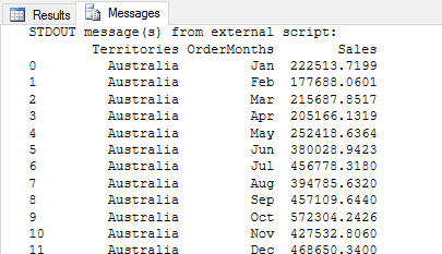
The first column, which is unnamed, is the data frame’s index. As with Series objects, Python generates the index automatically, starting with 0; however, you can change the index, reset it, or designate one of the columns as the index. The important point to remember is that a data frame, by default, is automatically assigned an index, which can be a factor when manipulating and analyzing data.
The final statement in the Python script assigns the df2 variable to the OutputDataSet variable:
|
1 |
OutputDataSet = df2 |
The OutputDataSet variable is the default variable used to return the script’s data to a calling application. Like the InputDataSet variable, the OutputDataSet variable is defined as a DataFrame object. The implication of this is that, when working with Python in SQL Server, you must pass your data to the OutputDataSet variable as a DataFrame object in order to return that data to a calling application. The following figure shows part of the data set returned by the OutputDataSet variable.
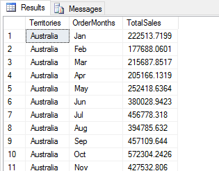
The integers shown in the first column are the row number labels used by SSMS. These values are not the index. The index is not included in the results. To include the index in the OutputDataSet results, you should use the reset_index function to turn that index into a column. For example, you can include the following statement in your script:
|
1 |
df2.reset_index(inplace=True) |
The reset_index function turns the existing index into a column and generates a new index. For this example, the function takes only the inplace argument, which is available to a number of functions. When set to True, the argument tells Python to update the data frame in place, without needing to reassign the data frame to itself or assign it to a new variable.
Also note that the results shown in the above figure include the Territories and OrderMonths columns. If you had set the as_index argument to True or had not included the argument when calling the groupby function, the results would include only the TotalSales column.
You can retrieve information about a data frame by calling its properties. For example, the following Python script retrieves the column names and dimensions of the df2 data frame:
|
1 2 3 4 5 6 7 8 9 10 11 12 13 14 15 16 17 18 19 20 21 22 23 24 25 26 27 28 29 |
DECLARE @pscript NVARCHAR(MAX); SET @pscript = N' import calendar as cl # calculate sales totals for each territory and month df1 = InputDataSet df2 = df1.groupby(["Territories", "OrderMonths"], as_index=False).sum() # change month numbers to abbreviated month names df2["OrderMonths"] = df2["OrderMonths"].apply(lambda x: cl.month_abbr[x]) # return information about data df2 data frame print(list(df2.columns.values)) print(df2.shape) print(len(df2.index))'; DECLARE @sqlscript NVARCHAR(MAX); SET @sqlscript = N' SELECT t.Name AS Territories, MONTH(h.OrderDate) AS OrderMonths, CAST(h.Subtotal AS FLOAT) AS Sales FROM Sales.SalesOrderHeader h INNER JOIN Sales.SalesTerritory t ON h.TerritoryID = t.TerritoryID WHERE YEAR(h.OrderDate) = 2013;'; EXEC sp_execute_external_script @language = N'Python', @script = @pscript, @input_data_1 = @sqlscript; GO |
The first print statement uses the list function and columns.values property to return a list of the columns in the df2 data frame. The shape property returns the data frame’s dimensions (number of rows and columns). The index property returns the data frame’s index. If you use the index property in conjunction with the len function, you’ll get the number of values in the index. (The len function returns the number of items in an object.) The Python scripts returns the following results:
|
1 2 3 |
['Territories', 'OrderMonths', 'Sales'] (120, 3) 120 |
The DataFrame class supports a wide range of properties (attributes) and functions (methods), making it possible to work with data in a variety of ways. For more information about the DataFrame class, see the topic pandas.DataFrame in the pandas documentation.
Adding columns to a data frame
Whether your data frames are based on SQL Server data or come from another source (or are a combination of both), there might be times when you’ll want to add columns. One way to do this is to aggregate the same source column in two different ways when calling the groupby function, as shown in the following example:
|
1 2 3 4 5 6 7 8 9 10 11 12 13 14 15 16 17 18 19 20 21 22 23 24 25 26 27 28 29 30 |
DECLARE @pscript NVARCHAR(MAX); SET @pscript = N' import calendar as cl # calculate sales averages and totals for each territory and month df1 = InputDataSet df2 = df1.groupby(["Territories", "OrderMonths"], as_index=False).agg({"Sales": ["mean", "sum"]}) # change month numbers to abbreviated month names df2["OrderMonths"] = df2["OrderMonths"].apply(lambda x: cl.month_abbr[x]) # return df2 data set OutputDataSet = df2'; DECLARE @sqlscript NVARCHAR(MAX); SET @sqlscript = N' SELECT t.Name AS Territories, MONTH(h.OrderDate) AS OrderMonths, CAST(h.Subtotal AS FLOAT) AS Sales FROM Sales.SalesOrderHeader h INNER JOIN Sales.SalesTerritory t ON h.TerritoryID = t.TerritoryID WHERE YEAR(h.OrderDate) = 2013;'; EXEC sp_execute_external_script @language = N'Python', @script = @pscript, @input_data_1 = @sqlscript WITH RESULT SETS((Territories NVARCHAR(100), OrderMonths NCHAR(3), AvgSales MONEY, TotalSales MONEY)); GO |
You should call the groupby function just like you did in the previous examples, but rather than tagging on the sum aggregate function at the end of the groupby function call, you specify the agg function, passing in a dictionary (dict) value as an argument. The dictionary value specifies the Sales column and two aggregate functions, mean and sum. The following figure shows part of the results that the Python script returns.
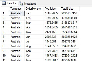
The data set now includes the AvgSales and TotalSales column, which are both based on the Sales column in the df1 data frame.
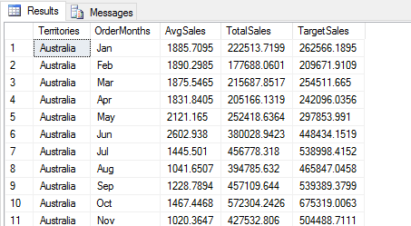
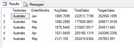
You can also insert columns into a data frame more directly, without having to define another aggregation. For example, the following Python script generates TargetSales sales, a computed column that adds 18% to the TotalSales values:
|
1 2 3 4 5 6 7 8 9 10 11 12 13 14 15 16 17 18 19 20 21 22 23 24 25 26 27 28 29 30 31 32 33 34 |
DECLARE @pscript NVARCHAR(MAX); SET @pscript = N' import calendar as cl # calculate sales averages and totals for each territory and month df1 = InputDataSet df2 = df1.groupby(["Territories", "OrderMonths"], as_index=False).agg({"Sales": ["mean", "sum"]}) # assign column names and add computed column df2.columns = ["Territories", "OrderMonths", "AvgSales", "TotalSales"] df2["TargetSales"] = df2["TotalSales"] * 1.18 # change month numbers to abbreviated month names df2["OrderMonths"] = df2["OrderMonths"].apply(lambda x: cl.month_abbr[x]) # return df2 data set OutputDataSet = df2'; DECLARE @sqlscript NVARCHAR(MAX); SET @sqlscript = N' SELECT t.Name AS Territories, MONTH(h.OrderDate) AS OrderMonths, CAST(h.Subtotal AS FLOAT) AS Sales FROM Sales.SalesOrderHeader h INNER JOIN Sales.SalesTerritory t ON h.TerritoryID = t.TerritoryID WHERE YEAR(h.OrderDate) = 2013;'; EXEC sp_execute_external_script @language = N'Python', @script = @pscript, @input_data_1 = @sqlscript WITH RESULT SETS((Territories NVARCHAR(100), OrderMonths NCHAR(3), AvgSales MONEY, TotalSales MONEY, TargetSales MONEY)); GO |
Before adding the column, I assigned names to the columns in the df2 data frame. I took this step to make it easier to reference those columns later in the script, which is especially beneficial when working with aggregated columns. (The pandas library also provides methods for naming aggregated and non-aggregated columns individually, but we’ll save that topic for a separate discussion.)
Instead of naming columns, you can reference columns by their internal index, but that can sometimes add more complexity than necessary. Personally, I prefer the readability that comes with using actual names.
To add column labels, first call the columns property on the df2 data frame and then assign the appropriate values to the property, providing each column name in the order the columns appears. You should enclose the column names in brackets and separate them with commas.
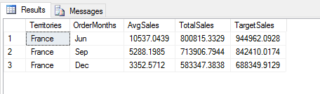
After renaming the columns, you can add the new column. Start by specifying the df2 data frame, followed by the new column name in brackets. Then set its value to an expression that calculates the values for the new column. In the example above, the expression simply multiples the TotalSales values by 1.18. The following figures shows part of the results now returned by the Python script.
Whenever you change your data frame in a way that will impact the columns retuned by the Python script, be sure to update the WITH RESULT SETS clause as necessary when calling the sp_execute_external_script stored procedure.
Filtering data in a data frame
The pandas library provides a variety of methods for filtering your data frame. For example, the following Python script uses the head function to return the first five rows from the data set:
|
1 2 3 4 5 6 7 8 9 10 11 12 13 14 15 16 17 18 19 20 21 22 23 24 25 26 27 28 29 30 31 32 33 34 |
DECLARE @pscript NVARCHAR(MAX); SET @pscript = N' import calendar as cl # calculate sales averages and totals for each territory and month df1 = InputDataSet df2 = df1.groupby(["Territories", "OrderMonths"], as_index=False).agg({"Sales": ["mean", "sum"]}) # assign column names and add computed column df2.columns = ["Territories", "OrderMonths", "AvgSales", "TotalSales"] df2["TargetSales"] = df2["TotalSales"] * 1.18 # change month numbers to abbreviated month names df2["OrderMonths"] = df2["OrderMonths"].apply(lambda x: cl.month_abbr[x]) # return top five rows OutputDataSet = df2.head(5)'; DECLARE @sqlscript NVARCHAR(MAX); SET @sqlscript = N' SELECT t.Name AS Territories, MONTH(h.OrderDate) AS OrderMonths, CAST(h.Subtotal AS FLOAT) AS Sales FROM Sales.SalesOrderHeader h INNER JOIN Sales.SalesTerritory t ON h.TerritoryID = t.TerritoryID WHERE YEAR(h.OrderDate) = 2013;'; EXEC sp_execute_external_script @language = N'Python', @script = @pscript, @input_data_1 = @sqlscript WITH RESULT SETS((Territories NVARCHAR(100), OrderMonths NCHAR(3), AvgSales MONEY, TotalSales MONEY, TargetSales MONEY)); GO |
To call the head function, you need only tag it onto the DataFrame object, optionally specifying the number of rows to return. If you don’t specify a number, Python will return five rows. The following figures shows the results returned by the Python script.
The pandas library also includes the tail function, which works the same way as the head function, except that it filters out all but the last rows in the data frame, instead of the first.
You can also specify which columns to retain in a data set:
|
1 2 3 4 5 6 7 8 9 10 11 12 13 14 15 16 17 18 19 20 21 22 23 24 25 26 27 28 29 30 31 32 33 |
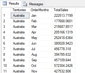
DECLARE @pscript NVARCHAR(MAX); SET @pscript = N' import calendar as cl # calculate sales averages and totals for each territory and month df1 = InputDataSet df2 = df1.groupby(["Territories", "OrderMonths"], as_index=False).agg({"Sales": ["mean", "sum"]}) # assign column names and add computed column df2.columns = ["Territories", "OrderMonths", "AvgSales", "TotalSales"] df2["TargetSales"] = df2["TotalSales"] * 1.18 # change month numbers to abbreviated month names df2["OrderMonths"] = df2["OrderMonths"].apply(lambda x: cl.month_abbr[x]) # return specific columns OutputDataSet = df2[["Territories", "OrderMonths", "TotalSales"]]'; DECLARE @sqlscript NVARCHAR(MAX); SET @sqlscript = N' SELECT t.Name AS Territories, MONTH(h.OrderDate) AS OrderMonths, CAST(h.Subtotal AS FLOAT) AS Sales FROM Sales.SalesOrderHeader h INNER JOIN Sales.SalesTerritory t ON h.TerritoryID = t.TerritoryID WHERE YEAR(h.OrderDate) = 2013;'; EXEC sp_execute_external_script @language = N'Python', @script = @pscript, @input_data_1 = @sqlscript WITH RESULT SETS((Territories NVARCHAR(100), OrderMonths NCHAR(3), TotalSales MONEY)); GO |
When including multiple columns, enclose them in a second set of brackets and separate the column names with commas. Python will then filter out all but the specified columns. The following figure shows part of the script’s results.
You can also add the head or tail function after specifying other filter criteria:
|
1 2 3 4 5 6 7 8 9 10 11 12 13 14 15 16 17 18 19 20 21 22 23 24 25 26 27 28 29 30 31 32 33 |
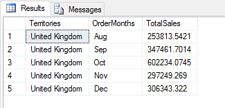
DECLARE @pscript NVARCHAR(MAX); SET @pscript = N' import calendar as cl # calculate sales averages and totals for each territory and month df1 = InputDataSet df2 = df1.groupby(["Territories", "OrderMonths"], as_index=False).agg({"Sales": ["mean", "sum"]}) # assign column names and add computed column df2.columns = ["Territories", "OrderMonths", "AvgSales", "TotalSales"] df2["TargetSales"] = df2["TotalSales"] * 1.18 # change month numbers to abbreviated month names df2["OrderMonths"] = df2["OrderMonths"].apply(lambda x: cl.month_abbr[x]) # return specific columns, last five rows OutputDataSet = df2[["Territories", "OrderMonths", "TotalSales"]].tail(5)'; DECLARE @sqlscript NVARCHAR(MAX); SET @sqlscript = N' SELECT t.Name AS Territories, MONTH(h.OrderDate) AS OrderMonths, CAST(h.Subtotal AS FLOAT) AS Sales FROM Sales.SalesOrderHeader h INNER JOIN Sales.SalesTerritory t ON h.TerritoryID = t.TerritoryID WHERE YEAR(h.OrderDate) = 2013;'; EXEC sp_execute_external_script @language = N'Python', @script = @pscript, @input_data_1 = @sqlscript WITH RESULT SETS((Territories NVARCHAR(100), OrderMonths NCHAR(3), TotalSales MONEY)); GO |
Now the returned data set includes only three columns and last five rows, as shown in the following figure.
In addition to columns, you can filter rows out of a data frame, based on conditional expressions you specify when calling the columns. For example, the following statement filters out all rows except those with a Territories value of France and TotalSales value greater than 500000:
|
1 2 3 4 5 6 7 8 9 10 11 12 13 14 15 16 17 18 19 20 21 22 23 24 25 26 27 28 29 30 31 32 33 34 |
DECLARE @pscript NVARCHAR(MAX); SET @pscript = N' import calendar as cl # calculate sales averages and totals for each territory and month df1 = InputDataSet df2 = df1.groupby(["Territories", "OrderMonths"], as_index=False).agg({"Sales": ["mean", "sum"]}) # assign column names and add computed column df2.columns = ["Territories", "OrderMonths", "AvgSales", "TotalSales"] df2["TargetSales"] = df2["TotalSales"] * 1.18 # change month numbers to abbreviated month names df2["OrderMonths"] = df2["OrderMonths"].apply(lambda x: cl.month_abbr[x]) # return specific rows OutputDataSet = df2[(df2["Territories"] == "France") & (df2["TotalSales"] > 500000)]'; DECLARE @sqlscript NVARCHAR(MAX); SET @sqlscript = N' SELECT t.Name AS Territories, MONTH(h.OrderDate) AS OrderMonths, CAST(h.Subtotal AS FLOAT) AS Sales FROM Sales.SalesOrderHeader h INNER JOIN Sales.SalesTerritory t ON h.TerritoryID = t.TerritoryID WHERE YEAR(h.OrderDate) = 2013;'; EXEC sp_execute_external_script @language = N'Python', @script = @pscript, @input_data_1 = @sqlscript WITH RESULT SETS((Territories NVARCHAR(100), OrderMonths NCHAR(3), AvgSales MONEY, TotalSales MONEY, TargetSales MONEY)); GO |
The first expression compares the Territories values to France, using the equals (==) comparison operator. The second expression compares the TotalSales values to 500000, using the greater than (>) comparison operator. Each expression is enclosed in parentheses and separated with the and (&) conditional operator, which indicates that both expressions must evaluate to true for a row to be included in the results, as shown in the following figure.

As an alternative to what we’ve seen so far, the pandas library provides a set of functions that also make it possible to filter data in a data frame. The functions include at, iat, loc, and iloc. The pandas documentation recommends using these functions when possible because they are optimized for data access. For information about these functions, see the pandas document Indexing and Selecting Data.
One of the most valuable of these functions is loc, which lets you filter out columns, rows, or both. The following syntax provides a simple overview of how to use the function:
|
1 |
<DataFrame>.loc[<rows>, <columns>] |
You specify row information as the first argument and column information as the second argument, separating the two by a comma. If you specify column information without row information, you need only include a colon for the first argument:
|
1 2 3 4 5 6 7 8 9 10 11 12 13 14 15 16 17 18 19 20 21 22 23 24 25 26 27 28 29 30 31 32 33 |
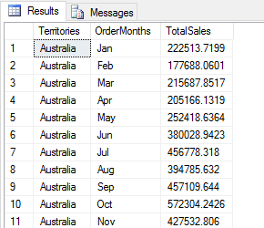
DECLARE @pscript NVARCHAR(MAX); SET @pscript = N' import calendar as cl # calculate sales averages and totals for each territory and month df1 = InputDataSet df2 = df1.groupby(["Territories", "OrderMonths"], as_index=False).agg({"Sales": ["mean", "sum"]}) # assign column names and add computed column df2.columns = ["Territories", "OrderMonths", "AvgSales", "TotalSales"] df2["TargetSales"] = df2["TotalSales"] * 1.18 # change month numbers to abbreviated month names df2["OrderMonths"] = df2["OrderMonths"].apply(lambda x: cl.month_abbr[x]) # return specific columns OutputDataSet = df2.loc[:,["Territories", "OrderMonths", "TotalSales"]]'; DECLARE @sqlscript NVARCHAR(MAX); SET @sqlscript = N' SELECT t.Name AS Territories, MONTH(h.OrderDate) AS OrderMonths, CAST(h.Subtotal AS FLOAT) AS Sales FROM Sales.SalesOrderHeader h INNER JOIN Sales.SalesTerritory t ON h.TerritoryID = t.TerritoryID WHERE YEAR(h.OrderDate) = 2013;'; EXEC sp_execute_external_script @language = N'Python', @script = @pscript, @input_data_1 = @sqlscript WITH RESULT SETS((Territories NVARCHAR(100), OrderMonths NCHAR(3), TotalSales MONEY)); GO |
The statement filters out all but the Territories, OrderMonths, and TotalSales columns. The following figure shows part of the results returned by the Python script.
If you want to filter out only rows, you can use the colon placeholder for the second argument or leave it off altogether. The following example includes the placeholder:
|
1 2 3 4 5 6 7 8 9 10 11 12 13 14 15 16 17 18 19 20 21 22 23 24 25 26 27 28 29 30 31 32 33 34 35 |
DECLARE @pscript NVARCHAR(MAX); SET @pscript = N' import calendar as cl # calculate sales averages and totals for each territory and month df1 = InputDataSet df2 = df1.groupby(["Territories", "OrderMonths"], as_index=False).agg({"Sales": ["mean", "sum"]}) # assign column names and add computed column df2.columns = ["Territories", "OrderMonths", "AvgSales", "TotalSales"] df2["TargetSales"] = df2["TotalSales"] * 1.18 # change month numbers to abbreviated month names df2["OrderMonths"] = df2["OrderMonths"].apply(lambda x: cl.month_abbr[x]) # return specific rows OutputDataSet = df2.loc[(df2["Territories"] == "France") & (df2["TotalSales"] > 500000),:]'; DECLARE @sqlscript NVARCHAR(MAX); SET @sqlscript = N' SELECT t.Name AS Territories, MONTH(h.OrderDate) AS OrderMonths, CAST(h.Subtotal AS FLOAT) AS Sales FROM Sales.SalesOrderHeader h INNER JOIN Sales.SalesTerritory t ON h.TerritoryID = t.TerritoryID WHERE YEAR(h.OrderDate) = 2013;'; EXEC sp_execute_external_script @language = N'Python', @script = @pscript, @input_data_1 = @sqlscript WITH RESULT SETS((Territories NVARCHAR(100), OrderMonths NCHAR(3), AvgSales MONEY, TotalSales MONEY, TargetSales MONEY)); GO |
Now the script returns all columns, but only few rows, as shown in the following figure.
To filter out both rows and columns, you can include both sets of criteria in one statement when using loc:
|
1 2 3 4 5 6 7 8 9 10 11 12 13 14 15 16 17 18 19 20 21 22 23 24 25 26 27 28 29 30 31 32 33 34 |
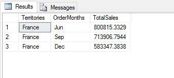
DECLARE @pscript NVARCHAR(MAX); SET @pscript = N' import calendar as cl # calculate sales averages and totals for each territory and month df1 = InputDataSet df2 = df1.groupby(["Territories", "OrderMonths"], as_index=False).agg({"Sales": ["mean", "sum"]}) # assign column names and add computed column df2.columns = ["Territories", "OrderMonths", "AvgSales", "TotalSales"] df2["TargetSales"] = df2["TotalSales"] * 1.18 # change month numbers to abbreviated month names df2["OrderMonths"] = df2["OrderMonths"].apply(lambda x: cl.month_abbr[x]) # return specific columns and rows OutputDataSet = df2.loc[(df2["Territories"] == "France") & (df2["TotalSales"] > 500000), ["Territories", "OrderMonths", "TotalSales"]]'; DECLARE @sqlscript NVARCHAR(MAX); SET @sqlscript = N' SELECT t.Name AS Territories, MONTH(h.OrderDate) AS OrderMonths, CAST(h.Subtotal AS FLOAT) AS Sales FROM Sales.SalesOrderHeader h INNER JOIN Sales.SalesTerritory t ON h.TerritoryID = t.TerritoryID WHERE YEAR(h.OrderDate) = 2013;'; EXEC sp_execute_external_script @language = N'Python', @script = @pscript, @input_data_1 = @sqlscript WITH RESULT SETS((Territories NVARCHAR(100), OrderMonths NCHAR(3), TotalSales MONEY)); GO |
As the following figure shows, the results are now leaner still.
Be sure to review the pandas documentation for more information about the different ways you can filter data in a data set. Consider what we’ve covered here as only the beginning.
Adding rows to a data frame
Earlier in this article, you saw how to add columns to your data frame. With pandas, you can also add rows. In the following example, the Python script generates a new data frame based on filtered data and then adds a row to the data frame:
|
1 2 3 4 5 6 7 8 9 10 11 12 13 14 15 16 17 18 19 20 21 22 23 24 25 26 27 28 29 30 31 32 33 34 35 36 37 38 39 40 |
DECLARE @pscript NVARCHAR(MAX); SET @pscript = N' import calendar as cl # calculate sales averages and totals for each territory and month df1 = InputDataSet df2 = df1.groupby(["Territories", "OrderMonths"], as_index=False).agg({"Sales": ["mean", "sum"]}) # assign column names and add computed column df2.columns = ["Territories", "OrderMonths", "AvgSales", "TotalSales"] df2["TargetSales"] = df2["TotalSales"] * 1.18 # change month numbers to abbreviated month names df2["OrderMonths"] = df2["OrderMonths"].apply(lambda x: cl.month_abbr[x]) # define the df3 data frame and add row df3 = df2.loc[(df2["OrderMonths"] == "Jun") & (df2["TotalSales"] > 500000), ["Territories", "AvgSales", "TotalSales"]] row = ["Australia", 8257.1674, 830092.7536] df3.loc[len(df3)] = row df3 = df3.sort_values(by="Territories") # return the df3 data set OutputDataSet = df3'; DECLARE @sqlscript NVARCHAR(MAX); SET @sqlscript = N' SELECT t.Name AS Territories, MONTH(h.OrderDate) AS OrderMonths, CAST(h.Subtotal AS FLOAT) AS Sales FROM Sales.SalesOrderHeader h INNER JOIN Sales.SalesTerritory t ON h.TerritoryID = t.TerritoryID WHERE YEAR(h.OrderDate) = 2013;'; EXEC sp_execute_external_script @language = N'Python', @script = @pscript, @input_data_1 = @sqlscript WITH RESULT SETS((Territories NVARCHAR(100), AvgSales MONEY, TotalSales MONEY)); GO |
To create the new data frame, the script uses the loc function to filter out all rows except those with an OrderMonths value that equals Jun and a TotalSales value greater than 500000. The function also filters out all but the Territories, AvgSales, and TotalSales columns. The filtered results are then assigned to the df3 variable to create the new data frame.
After defining the df3 data frame, the script specifies the values for the new row and saves them to the row variable. The script then uses the loc and len functions to set the value of the new row. The len function returns the number of rows in the data frame, and the loc function interprets that number as an index value for the new row.
This works because the index starts with 0, so the highest index number before the row is added is 3. The new row is added with an index value of 4 because the index size is four. As a result, the new row is inserted after all the other rows, which means that the territory names are no longer in alphabetical order. To fix this, you can call the sort_values function on the df3 data frame, specifying the name of the Territories column. The Python script now returns that data set shown in the following figure.
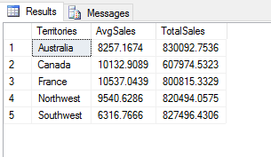
As you can see, the script returns a small data set that includes only five rows and three columns, just what we were after, with the values nicely sorted by territory name. The new row for Australia is included.
Removing a column from a data frame
You might also run into situations when you want to remove a column from a data frame. One way to do this is to use the loc function to filter out the column and then reassign the data frame to itself or a different variable. Another approach is to use the drop function available to the DataFrame class, as shown in the following example:
|
1 2 3 4 5 6 7 8 9 10 11 12 13 14 15 16 17 18 19 20 21 22 23 24 25 26 27 28 29 30 31 32 33 34 |
DECLARE @pscript NVARCHAR(MAX); SET @pscript = N' import calendar as cl # define the df1 data frame df1 = InputDataSet.groupby(["Territories", "OrderMonths"], as_index=False).agg({"Sales": ["mean", "sum"]}) df1.columns = ["Territories", "OrderMonths", "AvgSales", "TotalSales"] df1["TargetSales"] = df1["TotalSales"] * 1.18 df1["OrderMonths"] = df1["OrderMonths"].apply(lambda x: cl.month_abbr[x]) df1 = df1.loc[df1["TotalSales"] > 800000] df1 = df1.sort_values(by="TotalSales", ascending=False) # remove AvgSales column df1.drop("AvgSales", axis=1, inplace=True) # return df1 data set OutputDataSet = df1'; DECLARE @sqlscript NVARCHAR(MAX); SET @sqlscript = N' SELECT t.Name AS Territories, MONTH(h.OrderDate) AS OrderMonths, CAST(h.Subtotal AS FLOAT) AS Sales FROM Sales.SalesOrderHeader h INNER JOIN Sales.SalesTerritory t ON h.TerritoryID = t.TerritoryID WHERE YEAR(h.OrderDate) = 2013;'; EXEC sp_execute_external_script @language = N'Python', @script = @pscript, @input_data_1 = @sqlscript WITH RESULT SETS((Territories NVARCHAR(100), OrderMonths NCHAR(3), TotalSales MONEY, TargetSales MONEY)); GO |
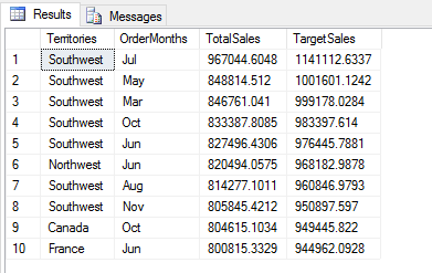
This time round, I consolidated some of the script, although at this point, you should be well familiar with most of these elements. The only new construct is the statement that uses the drop function to remove the AvgSales column.
When calling the function, first specify the name of the column that should be dropped. Next, add the axis argument, setting its value to 1. This indicates that you’re dropping a column, not the index (which would be 0). The inplace argument comes next. As you saw earlier, it tells Python to update the data frame in place. The Python script returns the data set shown in the following figure.
As the example demonstrates, the drop function provides yet another way to remove a column from a data frame. When working with pandas and Python, you’ll find that there are often a number of different ways to carry out a task. You might have to do some digging to figure out the best approach, but sometimes it’s just a matter of preference. The better you understand pandas and Python, the better you’ll understand the options you have available to work with the data.
Making the most of the data frame
There is, of course, a great deal more to data frames and the pandas library than what we’ve covered here, but this should provide you with a foundation for getting started so you can strike out on your own. The best way to acquaint yourself with Python, pandas, and data frames is to play around with data sets in your Python scripts and experiment with the various ways you can manipulate and analyze data.
As we progress through this series, we’ll dig more into the Python language and pandas library and some of ways you can work with data. Your understanding of data frames will be instrumental in your ability to move forward with MLS and Python and to perform advanced data analytics.
This document contains proprietary information and is protected by copyright law.
Copyright © 2026 Red Gate Software Limited. All rights reserved


Load comments