
The series so far:
- How to query blob storage with SQL using Azure Synapse
- How to query private blob storage with SQL and Azure Synapse
- Performance of querying blob storage with SQL
In the third part of the series Querying Blob Storage with SQL, I will focus on the performance behaviour of queries: What makes them faster, slower, and some syntax beyond the basics.
The performance tests in this article are repeated, and the best time of the queries is recorded. This doesn’t mean you will always achieve the same timing. Many architectural details will affect the timing, such as cache, first execution, and so on. The timing exposed on each query is only a reference pointing to the differences of the query methods that can affect the time and the usual result for better or worse performance.
Filtering data by filepath
Microsoft keeps some large datasets available for anyone to play with them using Synapse and other tools. The examples in this article use one of these datasets, the New York Yellow cab trips from many years.
Partitioning
Following Big Data rules, the detail rows about the taxi rides are broken down by year and month in different folders. It’s like partitioning the data.
You can query all folders, or partitions, at once by using wildcards in the query. The query below is a sample query summarizing the rides by year. Note that the query runs in Synapse Studio, which is part of the Synapse Workspace. See the previous articles to set up the workspace if it’s not already set up.
|
1 2 3 4 5 6 7 8 |
SELECT Year(tpepPickupDateTime), count(*) as Trips FROM OPENROWSET( BULK 'https://azureopendatastorage.blob.core.windows.net/nyctlc/yellow/puYear=*/puMonth=*/*.parquet', FORMAT='PARQUET' ) AS [nyc] group by Year(tpepPickupDateTime) |
The path may appear a bit strange, ‘puYear=’ and ‘puMonth=’ . These are part of the path. Only the wildcard symbol, ‘*’, replaces the year and month.
The source data has a date field, tpepPickupDateTime. This query above uses this field to summarize the years. The Synapse Serverless engine cannot tell that the Year used on the query is the same information hidden by wildcard on the path. That’s why it will read all the records.
Here are the execution results of the query:

Records: 29
Data Scanned: 19203MB (19GB)
Data Moved: 1 MB
Execution Time: 01:48.676
This query above does not make use of the folder partitioning at all; it’s just reading everything. Synapse Serverless has a function called FilePath that can use OPENROWSET to retrieve pieces of the path using wildcards. Each wildcard has a number, starting with 1, and the FilePath function can retrieve its value.
FilePath function
Replacing the year on the previous query by the FilePath function, the new query will look like this:
|
1 2 3 4 5 6 7 8 |
SELECT nyc.filepath(1) as Year, count(*) as Trips FROM OPENROWSET( BULK 'https://azureopendatastorage.blob.core.windows.net/nyctlc/yellow/puYear=*/puMonth=*/*.parquet', FORMAT='PARQUET' ) AS [nyc] group by nyc.filepath(1) |
This is the execution result of the new query:
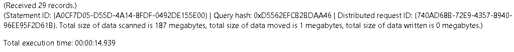
Records: 29
Data Scanned: 187 MB
Data Moved: 1 MB
Execution Time: 00:14.939
As you may notice, the first query takes over 1:30 longer than the second one. The second query reads less than half a gigabyte of data to retrieve the same amount of information and records and the exact same amount of content.
Using views to simplify the syntax
The OPENROWSET syntax can be quite long and complex, and adding the FilePath doesn’t make it easier.
The queries need to be easier to write so they can be used for those who will use Power BI or other BI tools, not only for those who will use the Serverless Pool directly to reach the Data Lake.
Views are a great solution to make the environment easier for our users. The Serverless Pool can’t hold tables, but you can create a database to host other objects, such as views.
It’s possible to build many different solutions using views, creating views with pre-defined queries to aggregate the data in different ways.
One of the most flexible ways to use the views in Synapse Serverless is to include the values of the FilePath in the view. By doing so, the users can use this value to create queries in Power BI using the partitioning schema built on the Data Lake. The users can also use these queries to configure aggregations in Power BI, turning a huge model into something possible to analyse in seconds.
The view can be created using the following query, but be sure to switch to the NYTaxi database if you are connected to master:
|
1 2 3 4 5 6 7 8 9 10 11 12 |
Create View Tripsvw AS SELECT vendorID,tpepPickupDateTime,tpepDropOffDateTime,passengerCount, tripDistance,puLocationId, doLocationId,startLon, startLat,endLon,endLat,rateCodeId,storeAndFwdFlag, paymentType, fareAmount, extra, mtaTax, improvementSurcharge,tipAmount ,tollsAmount, totalAmount, nyc.filepath(1) as Year,nyc.filepath(2) as Month FROM OPENROWSET( BULK 'https://azureopendatastorage.blob.core.windows.net/nyctlc/yellow/puYear=*/puMonth=*/*.parquet', FORMAT='PARQUET' ) AS [nyc] |
The preview query using FilePath can be simplified using the view:
|
1 2 3 4 5 |
SELECT Year, count(*) as Trips FROM Tripsvw group by Year |
How the schema affects performance
The previous article of this series demonstrated that the schema can be auto-detected or defined in the query. The method used and the schema defined can make a difference in the query performance.
For a matter of comparison, these different ways to build a query are considered:
- Auto-detect the schema
- Define a schema with the wrong size for the data types
- Define a schema with correct size but wrong string types, including collation
- Define a schema with the correct size and type, including collation
Besides these options for CSV types, all the options can be tested with both parsers except the auto-detect option, which only works with Parser 2.0:
- Parser 1.0
- Parser 2.0
Some file types, such as CSV, don’t have a schema at all, while other file types, such as PARQUET, don’t have the size of the fields.
Auto-detecting the schema has a name: Schema-on-Read. You can specify the schema while querying the data instead of the usual RDBMS, where you define the table schema when creating the table.
It’s common, when defining the schema, to make mistakes on the field sizes. Because the source files don’t hold the field sizes, this is hard to define. It’s also easy to make mistakes on the field types. Mistakes between varchar and nvarchar and integer types are very common.
The examples illustrate the performance implications of any mistake made on the field type when specifying a schema.
Defining the schema
Previous articles of this series showed how to use the procedure sp_describe_first_result_set to check the schema of a result set. Take a look at the example below:
|
1 2 3 4 5 |
sp_describe_first_result_set N'select top 10 * from OPENROWSET( BULK ''https://azureopendatastorage.blob.core.windows.net/holidaydatacontainer/Processed/'', FORMAT=''PARQUET'' ) AS [holidays] ' |
The result is shown in the image below. It contains field sizes but all the field sizes are their maximum size. The source files don’t have the size; it’s filled with the maximum size.
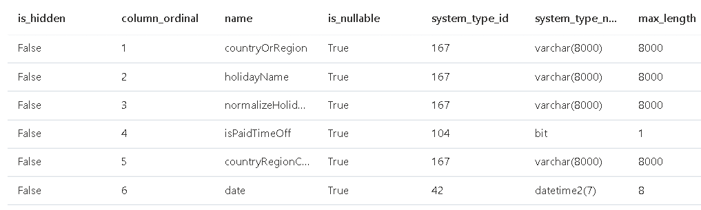
Using the maximum size on the schema definition is a usual mistake, exactly because these are the values returned on the schema specification. To discover the real size of the fields, use the query below:
|
1 2 3 4 5 6 7 8 |
select max(len(countryOrRegion)) AS maxCountryOrRegion, max(len(holidayName)) AS maxHolidayName, max(len(normalizeHolidayName)) AS maxNormalizedHolidayName, max(len(countryRegionCode)) AS maxCountryRegionCode from OPENROWSET( BULK 'https://azureopendatastorage.blob.core.windows.net/holidaydatacontainer/Processed/', FORMAT='PARQUET' ) AS [holidays] |
This is the result:

Parquet source files
The results can be analysed using a PARQUET data source.
Wrong type and size
|
1 2 3 4 5 6 7 8 9 10 11 12 13 14 |
select * from OPENROWSET( BULK 'https://azureopendatastorage.blob.core.windows.net/holidaydatacontainer/Processed/', FORMAT='PARQUET' ) WITH ( countryOrRegion varchar(8000), holidayName varchar(8000), normalizeHolidayName varchar(8000), isPaidTimeOff bit, countryRegionCode varchar(8000), date DATETIME2 ) AS [holidays] |
Correct size, wrong collation
|
1 2 3 4 5 6 7 8 9 10 11 12 13 14 |
select * from OPENROWSET( BULK 'https://azureopendatastorage.blob.core.windows.net/holidaydatacontainer/Processed/', FORMAT='PARQUET' ) WITH ( countryOrRegion varchar(16), holidayName varchar(170), normalizeHolidayName varchar(170), isPaidTimeOff bit, countryRegionCode char(2), date DATETIME2(7) ) AS [holidays] |
Solving collation with Unicode Strings
|
1 2 3 4 5 6 7 8 9 10 11 12 13 14 |
select * from OPENROWSET( BULK 'https://azureopendatastorage.blob.core.windows.net/holidaydatacontainer/Processed/', FORMAT='PARQUET' ) WITH ( countryOrRegion nvarchar(16), holidayName nvarchar(170), normalizeHolidayName nvarchar(170), isPaidTimeOff bit, countryRegionCode nchar(2), date DATETIME2(7) ) AS [holidays] |
Auto-detect
|
1 2 3 4 5 |
select * from OPENROWSET( BULK 'https://azureopendatastorage.blob.core.windows.net/holidaydatacontainer/Processed/', FORMAT='PARQUET' ) AS [holidays] |
Collation specified on string fields
|
1 2 3 4 5 6 7 8 9 10 11 12 13 14 |
select * from OPENROWSET( BULK 'https://azureopendatastorage.blob.core.windows.net/holidaydatacontainer/Processed/', FORMAT='PARQUET' ) WITH ( countryOrRegion varchar(16) COLLATE Latin1_General_100_BIN2_UTF8, holidayName varchar(170) COLLATE Latin1_General_100_BIN2_UTF8, normalizeHolidayName varchar(170) COLLATE Latin1_General_100_BIN2_UTF8, isPaidTimeOff bit, countryRegionCode char(2) COLLATE Latin1_General_100_BIN2_UTF8, date DATETIME2(7) ) AS [holidays] |
Here are the results:
| Scenario | Data scanned | Data moved | Duration |
| Wrong size and type | 1MB | 5MB | 9.962 seconds |
| Correct size, wrong collation | 1MB | 5MB | 8.298 seconds |
| Solving collation with Unicode strings | 1MB | 8MB | 13.734 seconds |
| Auto-detect | 1MB | 5MB | 9.491 seconds |
| Collation specified on string fields | 1MB | 5MB | 8.755 seconds |
After all these comparisons, there are some interesting conclusions to make:
- Using Unicode string types hide the collation problem when reading strings, but it doubles the size of the string, resulting in a higher data movement and terrible performance.
- The auto-detect feature is quite efficient; it’s almost as good as the correct choice of data types.
- The difference between the query without collation specification and with collation specification is almost nothing. I would recommend specifying the collation.
- The scanned data is smaller than the moved data because the files are compressed.
External Tables
As you notice, the query with the schema becomes quite complex. Once again, it’s possible to make a solution, so the queries are easier for users.
The previous article of the series demonstrated External Data Sources and creating a database in Synapse Serverless. This example uses the same techniques:
First, create a new external data source:
|
1 2 3 4 5 |
CREATE EXTERNAL DATA SOURCE [msSource] WITH ( LOCATION = 'https://azureopendatastorage.blob.core.windows.net/' ); go |
You can create external tables to map the schema to a table. This table doesn’t exist physically on the Serverless Pool; it’s only a schema mapping for the external storage.
The next step is to create two additional objects: An external file that will specify the format of the files on the external storage and the external table, mapping the schema of the external files.
|
1 2 3 4 5 6 7 8 9 10 11 12 13 14 15 16 17 18 19 |
CREATE EXTERNAL FILE FORMAT parquetcompressed WITH ( FORMAT_TYPE = PARQUET, DATA_COMPRESSION = 'org.apache.hadoop.io.compress.SnappyCodec' ); Create external table [extHolidays] ( countryOrRegion varchar(16) COLLATE Latin1_General_100_BIN2_UTF8, holidayName varchar(170) COLLATE Latin1_General_100_BIN2_UTF8, normalizeHolidayName varchar(170) COLLATE Latin1_General_100_BIN2_UTF8, isPaidTimeOff bit, countryRegionCode char(2) COLLATE Latin1_General_100_BIN2_UTF8, date DATETIME2(7) ) WITH (LOCATION = N'holidaydatacontainer/Processed/', DATA_SOURCE = [msSource], FILE_FORMAT = [parquetcompressed]); go select * from [extHolidays] |
External Tables: Performance Comparison
The first limitation you may notice on external tables is the lack of support for the FilePath function. This is a severe limitation because often, the data will be partitioned by folders, like the earlier examples.
Besides this severe difference, compare the performance difference between External Tables and OPENROWSET function.
OPENROWSET method
|
1 2 3 4 5 6 7 8 9 10 11 12 13 14 |
select * from OPENROWSET( BULK 'https://azureopendatastorage.blob.core.windows.net/holidaydatacontainer/Processed/', FORMAT='PARQUET' ) WITH ( countryOrRegion varchar(16) COLLATE Latin1_General_100_BIN2_UTF8, holidayName varchar(170) COLLATE Latin1_General_100_BIN2_UTF8, normalizeHolidayName varchar(170) COLLATE Latin1_General_100_BIN2_UTF8, isPaidTimeOff bit, countryRegionCode char(2) COLLATE Latin1_General_100_BIN2_UTF8, date DATETIME2(7) ) AS [holidays] |
External table method
|
1 2 |
select * from [extHolidays] |
Here are the results:
| Scenario | Data scanned | Data moved | Duration |
| OPENROWSET | 1MB | 5MB | 8.459 seconds |
| External table | 1MB | 5MB | 8.314 seconds |
You may notice the results are quite similar, allowing us to use external tables to simplify OPENROWSET queries when the FilePath function is not needed.
CSV File Format: Comparing parser and auto-detect
When reading data from CSV files, the main difference is the parser used. Parser 2.0 may appear to be a logical choice because of some advantages, such as auto-detecting schema and because the appearance to be a more advanced version.
However, the two versions have different features and limitations, and you will find situations where Parser 1.0 will be needed.
Here’s a comparison of features of the two versions:
| Parser 1.0 | Parser 2.0 |
|
|
| Reference: https://docs.microsoft.com/en-us/azure/synapse-analytics/sql/develop-openrowset | |
My personal suggestion: Use Parser 2.0 unless some specific requirement appears for Parser 1.0.
CSV Parsers and Collation
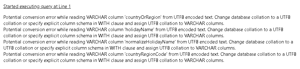
There are some differences between how Parsers 1.0 and 2.0 read strings. On our sample data, Parser 1.0 can read the string fields without much difficulty, while Parser 2.0 will require the correct collation specification or Unicode data type, increasing a bit the size of the field.
Synapse makes an automatic conversion from UTF8 collation to the collation used by string fields. In some situations, this automatic conversion may create problems on the data.
Parser 2.0, when used without a collation specification, results in a complaining message about collation, like you may notice on the image below.
When creating a database in Synapse Serverless, you can specify the collation as UTF8 using the following statement:
|
1 2 |
CREATE DATABASE mydb COLLATE Latin1_General_100_BIN2_UTF8; |
Another option is to change the collation in an existing database:
|
1 2 |
ALTER DATABASE mydb COLLATE Latin1_General_100_BIN2_UTF8; |
Besides defining the database collation, another option is to specify the collation of the string fields on the query schema. You need to discover if by doing so, you create some kind of performance difference.
Comparing the Performance
Here are some simple performance comparisons with the 4 possible situations:
- Using Parser 1.0 with schema
- Using Parser 2.0 with schema and collation
- Using Parser 2.0 with schema and nvarchar type
- Using Parser 2.0 auto-detecting fields
Using Parser 1.0 with schema
|
1 2 3 4 5 6 7 8 9 10 11 12 13 14 15 16 17 |
select * from OPENROWSET( BULK 'https://lakedemo.blob.core.windows.net/opendatalake/holidays/', FORMAT='CSV', FIELDTERMINATOR='|', firstrow=2, parser_version='1.0' ) WITH ( countryOrRegion varchar(16) COLLATE Latin1_General_100_BIN2_UTF8, holidayName varchar(225), normalizeHolidayName varchar(225), isPaidTimeOff bit, countryRegionCode char(2) COLLATE Latin1_General_100_BIN2_UTF8, date DATETIME2 ) AS [holidays] |
Using Parser 2.0 with schema and collation
|
1 2 3 4 5 6 7 8 9 10 11 12 13 14 15 16 17 |
select * from OPENROWSET( BULK 'https://lakedemo.blob.core.windows.net/opendatalake/holidays/', FORMAT='CSV', HEADER_ROW=true, FIELDTERMINATOR='|', parser_version='2.0' ) WITH ( countryOrRegion varchar(16) COLLATE Latin1_General_100_BIN2_UTF8, holidayName varchar(500) COLLATE Latin1_General_100_BIN2_UTF8, normalizeHolidayName varchar(500) COLLATE Latin1_General_100_BIN2_UTF8, isPaidTimeOff bit, countryRegionCode char(2) COLLATE Latin1_General_100_BIN2_UTF8, date DATETIME2 ) AS [holidays] |
Using Parser 2.0 with schema and nvarchar type
|
1 2 3 4 5 6 7 8 9 10 11 12 13 14 15 16 17 |
select * from OPENROWSET( BULK 'https://lakedemo.blob.core.windows.net/opendatalake/holidays/', FORMAT='CSV', HEADER_ROW=true, FIELDTERMINATOR='|', parser_version='2.0' ) WITH ( countryOrRegion nvarchar(16) COLLATE Latin1_General_100_BIN2_UTF8, holidayName nvarchar(225), normalizeHolidayName nvarchar(225), isPaidTimeOff bit, countryRegionCode nchar(2) COLLATE Latin1_General_100_BIN2_UTF8, date DATETIME2 ) AS [holidays] |
Using Parser 2.0 auto-detecting fields
|
1 2 3 4 5 6 7 8 |
select * from OPENROWSET( BULK 'https://lakedemo.blob.core.windows.net/opendatalake/holidays/', FORMAT='CSV', HEADER_ROW=true, FIELDTERMINATOR='|', parser_version='2.0' ) AS [holidays] |
Here are the results:
| Scenario | Data scanned | Data moved | Duration |
| Using Parser 1.0 with schema | 8MB | 5MB | 8.769 seconds |
| Using Parser 2.0 with schema and collation | 14MB | 6MB | 10.050 seconds |
| Using Parser 2.0 with schema and nvarchar type | 14MB | 9MB | 15.422 seconds |
| Using Parser 2.0 auto-detecting fields | 14MB | 6MB | 9.664 seconds |
The difference in the varchar fields causes processing overhead for the query. The auto-detect on Parser 2.0 manages this relatively well. Although still complaining about collation, it reaches a performance similar to Parser 1.0.
Conclusion
There are many variations about how to query files in a Data Lake. This article gives you some directions about how these variations can impact the query performance.
Additional Reference
Collation in Synapse Analytics: https://techcommunity.microsoft.com/t5/azure-synapse-analytics/always-use-utf-8-collations-to-read-utf-8-text-in-serverless-sql/ba-p/1883633


Load comments