Microsoft Fabric storage uses OneLake and Delta Tables, the core storage of all Fabric objects, as explained in my introduction to Microsoft Fabric.

Either if you use lakehouses, data warehouses, or even datasets, all the data is stored in the OneLake. OneLake uses Delta Tables as storage. In this way, we need to be aware of some “secrets” related to delta table storage in order to make the best decisions possible for our data platform solution.

Let’s analyze some of the Parquet and Delta Table behaviors.

Parquet and Delta

Parquet is an open source format which became famous as one of the most used formats in data lakes. It’s a columnar storage format intended to store historical data.

One very important “secret”, and the main subject of this blog is: Parquet format is immutable. It’s not possible to change the content of a Parquet file. It’s intended for historical data.

Although the main objective is for historical data, many people and companies worked on this problem. The result was Delta Tables.

Delta Tables use the Parquet format, it’s not a different format. The immutable behavior continues. However, Delta Tables use an additional folder as a transaction log. The operations are registered in the delta logs, marking records with updates and deletes.

In this way, the underlying immutable behavior is still present, but we can work with the data in a transactional way, allowing updates and deletes, for example.

Time Travel

The delta logs allow us to make what’s called Time Travel. We can retrieve the information from a delta table in the way it was on a specific date and time, as long as the logs are kept complete.

The access to the entire historical of data changes is an important resource for a data storage.

Data Modelling

The need to keep historical data is way older than technologies such as Delta Time Travel, which allow us to keep them. The Data Modelling techniques, such as Data Warehouse modelling, proposed solutions for historical storage a long time ago.

One of the features used for this purpose is called Slowly Changing Dimensions, or Dimension Type 2. When we design a start schema, we decide which dimensions should keep an entire history and which ones aren’t worth the trouble and a simple update on the records would be enough.

For example, let’s consider a dimension called Customer. If we decide to keep the dimension as a SCD dimension, every time a customer record is changed in production, we create a new version of the record in the intelligence storage (data warehouse, data lake, whatever the name).

On the other hand, if we decide that a dimension is not worth keeping a history, we can just update the record in the intelligence storage when needed.

The decision of using a SCD dimension or not, and many more, are all made during modelling. They are independent of any technical feature capable of keeping the history of the data. The history is designed during modelling and kept by us.

Choosing Between Time Travel and Data Modelling

We have the possibility to use data modelling to control the history of our storage, or use the technical features, such as Time Travel.

This leads to several possibilities with different consequences:

The decision whether we should rely on modelling, on technology or stay somewhere in the middle is complex enough to generate many books. What’s important on this blog is to understand the decision is present when designing an architecture with Microsoft Fabric.

In order to make a well-informed decision, we need to understand how the delta tables process updates/deletes.

Lakehouse Example

The example will be made using a table called Fact_Sale. You can use a pipeline to import the data from https://azuresynapsestorage.blob.core.windows.net/sampledata to the files area of one Fabric Lakehouse. The article about Lakehouse and ETL explains how to build a pipeline to bring data to the Files area.

The article https://www.red-gate.com/simple-talk/blogs/microsoft-fabric-using-notebooks-and-table-partitioning-to-convert-files-to-tables/ explains this import process and how we can partition the data by Year and Quarter, making a more interesting example. The notebook code to import the partitioned data to the Tables area of the lakehouse is the following:

from pyspark.sql.functions import col, year, month, quarter
table_name = 'fact_sale'
df = spark.read.format("parquet").load('Files/fact_sale_1y_full')
df = df.withColumn('Year', year(col("InvoiceDateKey")))
df = df.withColumn('Quarter', quarter(col("InvoiceDateKey")))
df = df.withColumn('Month', month(col("InvoiceDateKey")))
df.write.mode("overwrite").format("delta").partitionBy("Year","Quarter").save("Tables/" + table_name)

The default size for a Parquet file in the Fabric environment is 1GB (1073741824 bytes). This is defined by the session configuration spark.microsoft.delta.optimizeWrite.binSize and has the purpose to avoid the delta lake small files problem. Although this is a common problem, the writing on delta tables can cause consequences when the file is too big. Let’s analyze this as well.

You can find more about Spark configuration on this blog and more about the small files problem on this link.

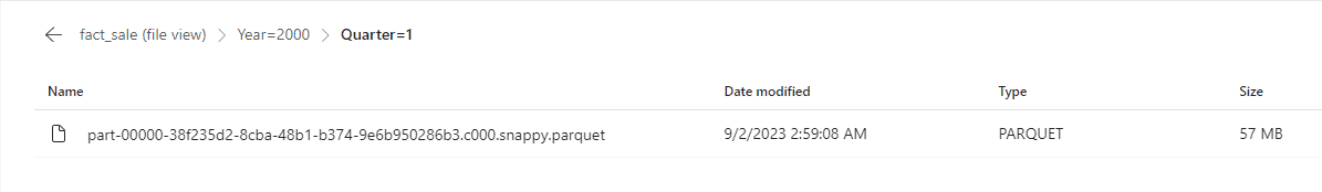
On our example, this configuration generated a single parquet file for each quarter, this will help to identify what’s happening during the example.

The Data we Have

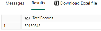
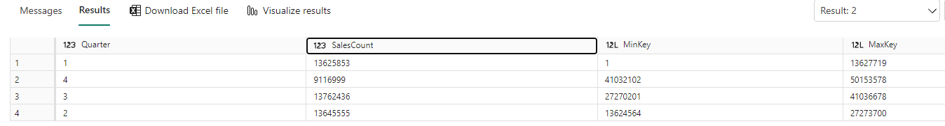
We need to identify the total of records we have, the total records for each quarter, and the minimum and maximum SalesKey value in each quarter in order to build the example.

We can use the SQL Endpoint to run the following queries:

Test query and Execution Time

For test purposes, let’s use the following query:

This query makes a grouping on all our records by CustomerKey, across the quarter partitions, creating a total of Sales by customer. On each test, I will execute this query 10 times and check the initial, minimum, and maximum execution time.

Updating one single record

As the first test, let’s update one single sales record in each quarter. We will use a notebook to execute the following code:

%%sql
update fact_sale set TotalIncludingTax=TotalIncludingTax * 2
where SaleKey = 6000000;

update fact_sale set TotalIncludingTax=TotalIncludingTax * 2
where SaleKey = 15624569 ;

update fact_sale set TotalIncludingTax=TotalIncludingTax * 2
where SaleKey = 35270205;

update fact_sale set TotalIncludingTax=TotalIncludingTax * 2
where SaleKey = 45032105;

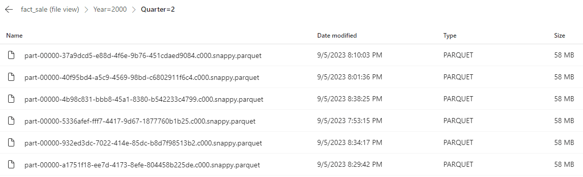
After executing these updates, if you look on the table Parquet files, you will notice each parquet file containing the record updated was duplicated.

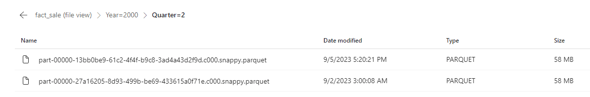
The parquet file continues to be immutable, in order to update a record, the entire file is duplicated with the record update and the delta logs register this update.

In our example, we updated 4 records, but each one was in a different parquet file. As a result, all the parquet files were duplicated (one for each quarter).

Remember the default file size is 1GB. A single record update will result in the duplication of a 1GB file. The big file size may have a bad side effect if you decide to use upserts or deletes too much.

Testing the Execution

Let’s test the execution of our sample query again and get the number after these duplication of parquet files:

There is a initial execution substantially slower and the average, even ignoring the initial execution, is slower, but not much.

Updating many records

Let’s change a bit the script and update a higher volume of records each quarter. You can execute the script below many times and each time you execute you will see the parquet files being duplicated.

%%sql
update fact_sale set TotalIncludingTax=TotalIncludingTax * 2
where SaleKey < 7000000;

update fact_sale set TotalIncludingTax=TotalIncludingTax * 2
where SaleKey > 14624564 AND SaleKey < 18624564;

update fact_sale set TotalIncludingTax=TotalIncludingTax * 2
where SaleKey > 28270201 AND SaleKey < 35270201;

update fact_sale set TotalIncludingTax=TotalIncludingTax * 2
where SaleKey > 42032102 AND SaleKey < 45032102;

Result

After executing the update script 4 times, we end up with 6 files on each partition. The original file, the file created by the update of a single record and the 4 files created when updating multiple record.

These are the results of the test query execution:

The test seems to illustrate only the initial query is affected and affected a lot. After the data is in cache, the files in the delta table don’t affect the query, or at least, it seems so.

On one hand, this illustrates the problem. On the other hand, we are talking about a few seconds difference for a set of 50 million records.

Cleaning the Table

The process of cleaning the table from unlinked parquet files is executed by the statement VACUUM. There are some important points to highlight about this process:

• If you decide to manage yourself the data history using data modelling, this needs to be a regular process on tables affected by updates and deletes.
• On the other hand, if you decide to use Time Travel to manage history, you can’t execute this process, otherwise you will lose the time travel capability.

This process needs to be executed very carefully. You can’t try to delete files while you have some process in execution over the data. You need to ensure this will only be executed while you don’t have anything running over the data.

The default method to ensure this is to only delete files older than one specific time. For example, if you want to delete unlinked files younger than 168 hours, you need to activate a special spark session configuration to ensure you are aware about what you are doing.

In this way, the example below, which activates this configuration and executes the VACUUM with 0 retention, is only for test purposes, not for production scenarios.

spark.conf.set("spark.databricks.delta.retentionDurationCheck.enabled", "false")

%%sql
VACUUM 'Tables/fact_sale' RETAIN 0 HOURS

After executing this cleaning, the additional files will disappear and only the most updated will remain.

Onelake is for all

This process affects not only the lakehouse, but the data warehouse as well. In the lakehouse, the SQL Endpoint is read-only, but the Data Warehouse is read-write with MERGE operations.

Conclusion

Microsoft Fabric is a PaaS environment for the entire Enterprise Data Architecture and capable of enabling the most modern architectures, such as Data Mesh.

However, we should never lose track of the data concepts, such as the fact the data intelligence storage is intended to be read-only and for historical purposes. Our architectural decisions may have an impact on the result which may not be so obvious in a PaaS environment.