
In previous articles in this SQL Server Integration Services (SSIS) series, we included several example SSIS packages that used the Data Flow task to retrieve data from a SQL Server databases and load that data into destination tables or files. Each data flow included at least one transformation component that somehow modified the data in order to prepare it for the destination.
In this article, we’ll look at another type of component: the Merge Join transformation. The Merge Join transformation lets us join data from more than one data source, such as relational databases or text files, into a single data flow that can then be inserted into a destination such as a SQL Server database table, Excel spreadsheet, text file, or other destination type. The Merge Join transformation is similar to performing a join in a Transact-SQL statement. However, by using SSIS, you can pull data from different source types. In addition, much of the work is performed in-memory, which can benefit performance under certain condition.
In this article, I’ll show you how to use the Merge Join transformation to join two tables from two databases into one data flow whose destination is a single table. Note, however, that although I retrieve data from the databases on a single instance of SQL Server, it’s certainly possible to retrieve data from different servers; simply adjust your connection settings as appropriate.
You can also use the Merge Join transformation to join data that you retrieve from Excel spreadsheets, text or comma-separated values (CSV) files, database tables, or other sources. However, each source that you join must include one or more columns that link the data in that source to the other source. For example, you might want to return product information from one source and manufacturer information from another source. To join this data, the product data will likely include an identifier, such as a manufacturer ID, that can be linked to a similar identifier in the manufacturer data, comparable to the way a foreign key relationship works between two tables. In this way, associated with each product is a manufacturer ID that maps to a manufacturer ID in the manufacturer data. Again, the Merge Join transformation is similar to performing a join in T-SQL, so keep that in mind when trying to understand the transformation.
Preparing the Source Data for the Data Flow
Before we actually set up our SSIS package, we should ensure we have the source data we need for our data flow operation. To that end, we need to two databases: Demo and Dummy. Of course, you do not need to use the same data structure that we’ll be using for this exercise, but if you want to follow the exercise exactly as described, you should first prepare your source data.
To help with this demo, I created the databases on my local server. I then copied data from the AdventureWorks2008 database into those databases. Listing 1 shows the T-SQL script I used to create the databases and their tables, as well as populate those tables with data.
|
1 2 3 4 5 6 7 8 9 10 11 12 13 14 15 16 17 18 19 20 21 22 23 24 25 26 27 28 29 30 31 32 33 34 35 36 37 38 39 40 41 |
USE master; GO IF DB_ID('Demo') IS NOT NULL DROP DATABASE Demo; GO CREATE DATABASE Demo; GO IF DB_ID('Dummy') IS NOT NULL DROP DATABASE Dummy; GO CREATE DATABASE Dummy; GO IF OBJECT_ID('Demo.dbo.Customer') IS NOT NULL DROP TABLE Demo.dbo.Customer; GO SELECT TOP 500 CustomerID, StoreID, AccountNumber, TerritoryID INTO Demo.dbo.Customer FROM AdventureWorks2008.Sales.Customer; IF OBJECT_ID('Dummy.dbo.Territory') IS NOT NULL DROP TABLE Dummy.dbo.Territory; GO SELECT TerritoryID, Name AS TerritoryName, CountryRegionCode AS CountryRegion, [Group] AS SalesGroup INTO Dummy.dbo.Territory FROM AdventureWorks2008.Sales.SalesTerritory; |
Listing 1: Creating the Demo and Dummy databases
As Listing 1 shows, I use a SELECT...INTO statement to create and populate the Customer table in the Demo database, using data from the Customer table in the AdventureWorks2008 database. I then use a SELECT...INTO statement to create and populate the Territory table in the Dummy database, using data from the SalesTerritory table in the AdventureWorks2008 database.
Creating Our Connection Managers
Once we’ve set up our source data, we can move on to the SSIS package itself. Our first step, then, is to create an SSIS package. Once we’ve done that, we can add two OLE DB connection managers, one to the Demo database and one to the Dummy database.
To create the first connection manager to the Demo database, right-click the Connection Manager window, and then click New OLE DB Connection, as shown in Figure 1.
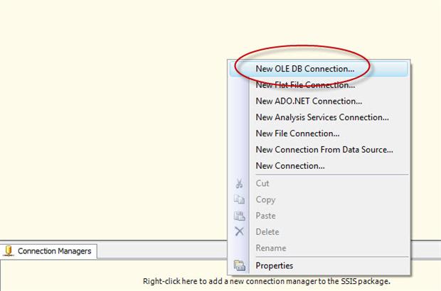
Figure 1: Creating an OLE DB connection manager
When the Configure OLE DB Connection Manager dialog box appears, click New. This launches the Connection Manager dialog box, where you can configure the various options with the necessary server and database details, as shown in Figure 2. (For this exercise, I created the Demo and Dummy databases on the ZOO-PC\CAMELOT SQL Server instance.)
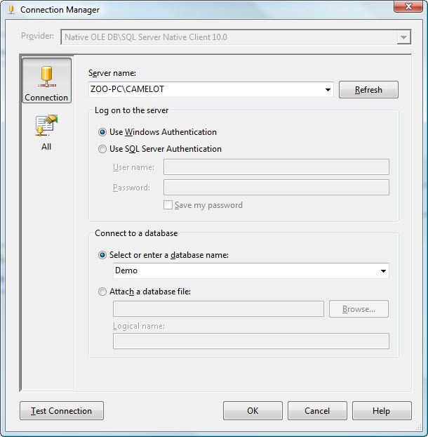
Figure 2: Configuring a new connection manager
After you’ve set up your connection manager, ensure that you’ve configured it correctly by clicking the Test Connection button. You should receive a message indicating that you have a successful connection. If not, check your settings.
Assuming you have a successful connection, click OK to close the Connection Manager dialog box. You’ll be returned to the Configure OLE DB Connection Manager dialog box. Your newly created connection should now be listed in the Data connections window.
Now create a connection manager for the Dummy database, following the same process that you used for the Demo database.
The next step, after adding the connection managers to our SSIS package, is to add a Data Flow task to the control flow. As you’ve seen in previous articles, the Data Flow task provides the structure necessary to add our components (sources, transformations, and destinations) to the data flow.
To add the Data Flow task to the control flow, drag the task from the Control Flow Items section of the Toolbox to the control flow design surface, as shown in Figure 3.
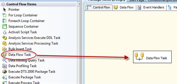
Figure 3: Adding a Data Flow task to the control flow
The Data Flow task serves as a container for other components. To access that container, double-click the task. This takes you to the design surface of the Data Flow tab. Here we can add our data flow components, starting with the data sources.
Adding Data Sources to the Data Flow
Because we’re retrieving our test data from two SQL Server databases, we need to add two OLE DB Source components to our data flow. First, we’ll add a source component for the Customer table in the Demo database. Drag the component from the Data Flow Source s section of the Toolbox to the data flow design surface.
Next, we need to configure the OLE DB Source component. To do so, double-click the component to open the OLE DB Source Editor, which by default, opens to the Connection Manager page.
We first need to select one of the connection managers we created earlier. From the OLE DB connection manager drop-down list, select the connection manager you created to the Demo database. On my system, the name of the connection manager is ZOO-PC\CAMELOT.Demo. Next, select the dbo.Customer table from the Name of the table or the view drop-down list. The OLE DB Source Editor should now look similar to the one shown in Figure 4.
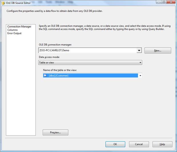
Figure 4: Configuring the OLE DB Source Editor
Now we need to select the columns we want to retrieve. Go to the Columns page and verify that all the columns are selected, as shown in Figure 5. These are the columns that will be included in the component’s output data flow. Note, however, if there are columns you don’t want to include, you should de-select those columns from the Available External Columns list. Only selected columns are displayed in the External Column list in the bottom grid. For this exercise, we’re using all the columns, so they should all be displayed.
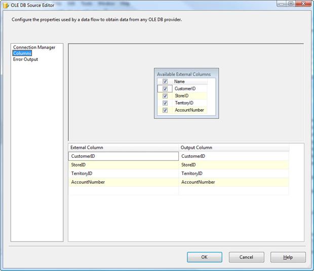
Figure 5: Selecting columns in the OLE DB Source Editor
Once you’ve verified that the correct columns have been selected, click OK to close the OLE DB Source Editor.
Now we must add an OLE DB Source component for the Territory table in the Dummy database. To add the component, repeat the process we’ve just walked through, only make sure you point to the correct database and table.
After we’ve added our source components, we can rename them to make it clear which one is which. In this case, I’ve renamed the first one Demo and the second one Dummy, as shown in Figure 6.
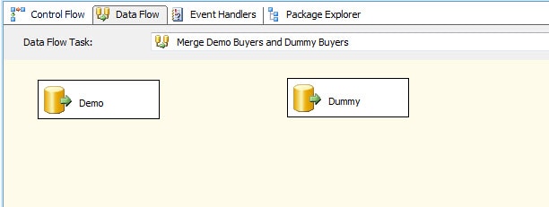
Figure 6: Setting up the OLE DB source components in your data flow
To rename the OLE DB Source component, right-click the component, click Rename, and then type the new name directly in the component.
Adding the Merge Join Transformation to the Data Flow
Now that we have the data sources, we can add the Merge Join transformation by dragging it from the Data Flow Transformations section of the Toolbox to the data flow design surface, beneath the source components, as shown in Figure 7.
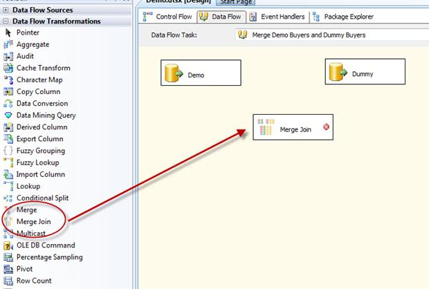
Figure 7: Adding the Merge Join transformation to the data flow
We now need to connect the data flow paths from the Demo and Dummy source components to the Merge Join transformation. First, drag the data path (green arrow) from the Demo source component to the Merge Join transformation. When you attach the arrow to the transformation, the Input Output Selection dialog box appears, displaying two options: the Output drop-down list and the Input drop-down list. The Output drop-down list defaults to OLE DB Source Output, which is what we want. From the Input drop-down list, select Merge Join Left Input, as shown in Figure 8. We’ll use the other option, Merge Join Right Input, for the Dummy connection.
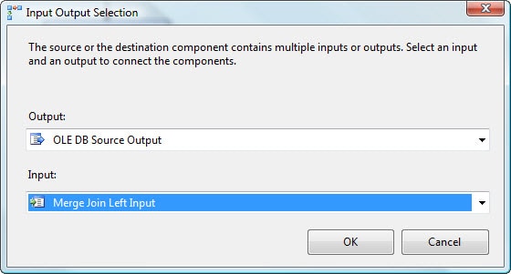
Figure 8: Configuring the Input Output Selection dialog box
Next, connect the data path from the Dummy data source to the Merge Join transformation. This time, the Input Output Selection dialog box does not appear. Instead, the Input drop-down list defaults to the only remaining option: Merge Join Right Input. Your data flow should now resemble the one shown in Figure 9.
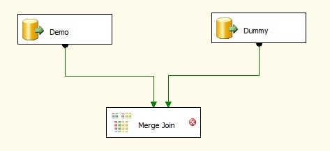
Figure 9: Connecting the source components to the Merge Join transformation
You may have noticed that a red circle with a white X is displayed on the Merge Join transformation, indicating that there is an error. If we were to run the package as it currently stands, we would receive the error message shown in Figure 10.
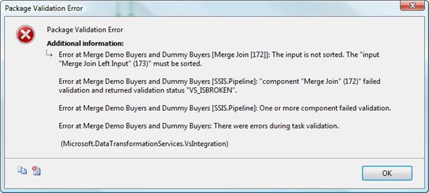
Figure 10: Receiving a package validation error on the Merge Join transformation
The reason for the error message is that the data being joined by a Merge Join transformation must first be sorted. There are two ways of achieving this: by sorting the data through the OLE DB S ource component or by adding a Sort transformation to the data flow.
Sorting Data Through the OLE DB Source
To sort the data through the OLE DB source component, you must first modify the connection to use a query, rather than specifying a table name. Double-click the Demo source component to open the OLE DB Source Editor. From the Data access mode drop-down list, select SQL command. Then, in the SQL command text window, type the following SELECT statement:
|
1 2 3 |
SELECT CustomerID, StoreID, AccountNumber, TerritoryID FROM dbo.Customer ORDER BY TerritoryID |
The Connection Manager page of the OLE DB Source Editor should now look similar to the one shown in Figure 11.
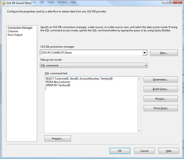
Figure 11: Defining a SELECT statement to retrieve data from the Customer table
Once you’ve set up your query, click OK to close the OLE DB Source Editor. You must then use the advanced editor of the OLE DB Source component to sort specific columns. To access the editor, right-click the component, and then click Show Advanced Editor.
When the Advanced Editor dialog box appears, go to the Input and Output Properties tab. In the Inputs and Outputs window, select the OLE DB Source Output node. This will display the Common Properties window on the right-hand side. In that window, set the IsSorted option to True, as shown in Figure 12.
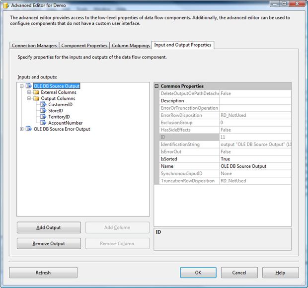
Figure 12: Configuring the IsSorted property on the Demo data source
We have told the package that the source data will be sorted, but we must now specify the column or columns on which that sort is based. To do this, expand the Output Columns subnode (under the OLE DB Source Output node), and then select TerritoryID column. The Common Properties window should now display the properties for that column. Change the value assigned to the SortKeyPosition property from 0 to a 1, as shown in Figure 13. The setting tells the other components in the data flow that the data is sorted based on the TerritoryID column. This setting must be consistent with how you’ve sorted your data in your query. If you want, you can add additional columns on which to base your sort, but for this exercise, the TerritoryID column is all we need.
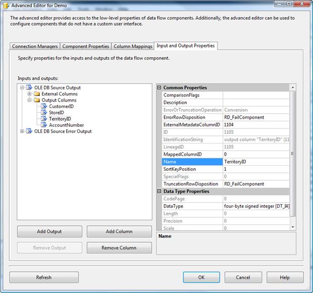
Figure 13: Configuring the SortKeyPosition property on the Territory ID column
Once you’ve configured sorting on the Demo data source, click OK to close the Advanced Editor dialog box.
Adding a Sort Transformation to the Data Flow
Another option for sorting data in the data flow is to use the Sort transformation. When working with an OLE DB Source component, you usually want to use the source component’s T-SQL query and advanced editor to sort the data. However, for other data sources, such as a text file, you won’t have this option. And that’s where the Sort transformation comes in.
Delete the data path that connects the Dummy data source to the Merge Join transformation by right-clicking the data path and then clicking Delete.
Next, drag the Sort transformation from the Data Flow Transformations section of the Toolbox to the data flow design surface, between the Dummy data source and the Merge Join transformation, as shown in Figure 14.
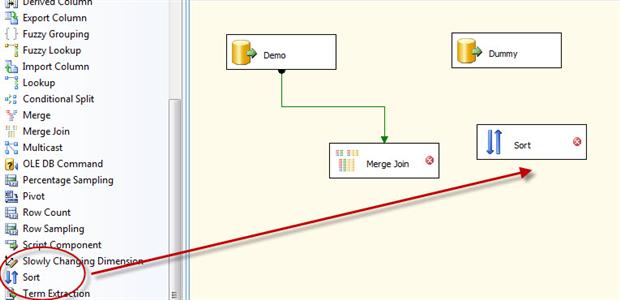
Figure 14: Adding the Sort transformation to the data flow
Drag the data path from the Dummy data source to the Sort transformation. Then double-click the Sort transformation to open the Sort Transformation Editor, shown in Figure 15.

Figure 15: Configuring the Sort transformation
As you can see in the figure, at the bottom of the Sort Transformation Editor there is a warning message indicating that we need to select at least one column for sorting. Select the checkbox to the left of the TerritoryID column in the Available Input Columns list. This adds the column to the bottom grid, which means the data will be sorted based on that column. By default, all other columns are treated as pass-through, which means that they’ll be passed down the data flow in their current state.
When we select a column to be sorted, the sort order and sort type are automatically populated. These can obviously be changed, but for our purposes they’re fine. You can also rename columns in the Output Alias column by overwriting what’s in this column.
Once you’ve configured the sort order, click OK to close the Sort Transformation Editor.
We now need to connect the Sort transformation to the Merge Join transformation, so drag the data path from the Sort transformation to the Merge Join transformation, as shown in Figure 16.
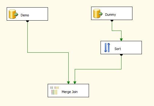
Figure 16: Connecting the Sort transformation to the Merge Join transformation
That’s all we need to do to sort the data. For the customer data, we used the Demo source component. For the territory data, we used a Sort transformation. As far as the Merge Join transformation is concerned, either approach is fine, although, as mentioned earlier, if you’re working with an OLE DB Source component, using that component is usually the preferred method.
Configuring the Merge Join Transformation
Now that we have our source data sorted and the data sources connected to the Merge Join transformation, we must now configure a few more settings of the Merge Join transformation.
Double-click the transformation to launch the Merge Join Transformation Editor, as shown in Figure 17.
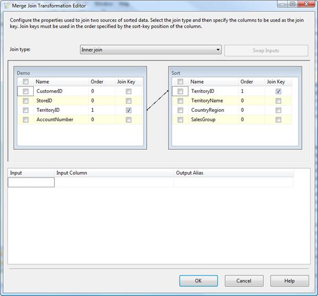
Figure 17: The default settings of the Merge Join Transformation Editor
Notice that your first setting in the Merge Join Transformation Editor is the Join type drop-down list. From this list, you can select one of the following three join types:
Left outer join: Includes all rows from the left table, but only matching rows from the right table. You can use theSwap Inputsoption to switch data source, effectively creating a right outer join.Full outer join: Includes all rows from both tables.Inner join: Includes rows only when the data matches between the two tables.
For our example, we want to include all rows from left table (Customer) but only rows from the right table (Territory) if there’s a match, so we’ll use the Left outer join option.
The next section in the Merge Join Transformation Editor contains the Demo grid and Sort Grid. The Demo grid displays the table from the Demo data source. The Sort grid displays the table from the Dummy data source. However, because the Sort transformation is used, the Sort transformation is considered the source of the data. Had we changed the output column names in the Sort transformation, those names would be used instead of the original ones.
Notice that an arrow connects the TerritoryID column in the Demo grid to that column in the Sort grid. SSIS automatically matches columns based on how the data has been sorted in the data flow. In this case, our sorts are based on the TerritoryID column in both data sources, so those columns are matched and serve as the basis of our join.
You now need to select which columns you want to include in the data set that will be outputted by the Merge Join transformation. For this exercise, we’ll include all columns except the AccountNumber column in the Customer table and the TerritoryID column from the Territory table. To include a column in the final result set, simply select the check box next to the column name in either data source, as shown in Figure 18.
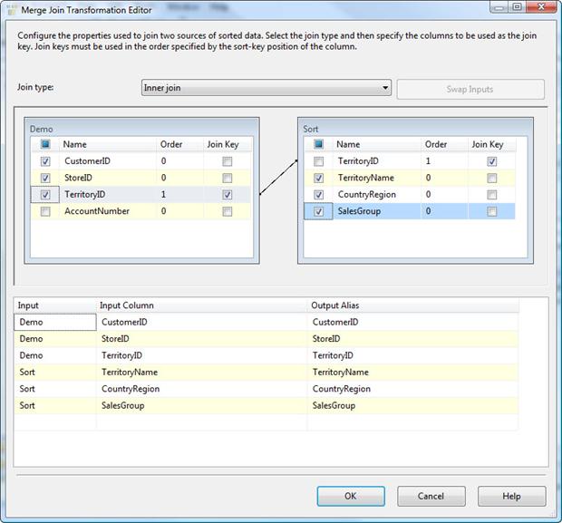
Figure 18: Specifying the columns to include in the merged result set
Notice that the columns you select are included in the lower windows. You can provide an output alias for each column if you want, but for this exercise, the default settings work fine.
Once you’ve configured the Merge Join transformation, click OK to close the dialog box. You’re now ready to add your data destination to the data flow.
Adding an OLE DB Destination to the Data Flow
Our final step in setting up the data flow is to add an OLE DB Destination component so that we can save our merged data to a new table. We’ll be using this component to add a table to the Demo database and populate the table with joined data. So drag the OLE DB Destination component from the Data Flow Destinations section of the Toolbox to the data flow design surface, beneath the Merge Join transformation, as shown in Figure 19.
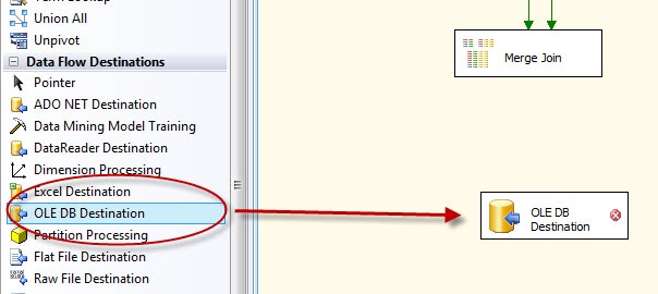
Figure 19: Adding an OLE DB Destination component to the data flow
We now need to connect the OLE DB Destination component to the Merge Join transformation by dragging the data path from the transformation to the destination. Next, double-click the destination to open the OLE DB Destination Editor.
On the Connection Manager page of the OLE DB Destination Editor, specify connection manager for the Demo database. Then, from the Data access mode drop-down list, select Table or view - fast load, if it’s not already selected.
Next, we’re going to create a target table to hold our result set. Click the New button next to the Name of the table or the view option and the Create Table dialog box opens. In it a table definition is automatically generated that reflects the columns passed down the data flow. You can rename the table (or any other element) by modifying the table definition. On my system, I renamed the table Me rge_Output, as shown in Figure 20, once you are happy with the table definition click on OK.
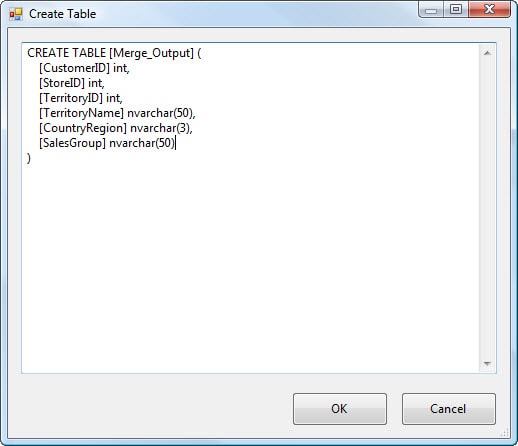
Figure 20: Using an OLE DB Destination component to create a table
Click on OK to close the Create Table dialog box. When you’re returned to the OLE DB Destination Editor, go to the Mappings page and ensure that your columns are all properly mapped. (Your results should include all columns passed down the pipeline, which should be the default settings.) Click OK to close the OLE DB Destination Editor. We have now set up a destination so all that’s left to do is to run it and see what we end up with.
Running Your SSIS Package
Your SSIS package should now be complete. The next step is to run it to make sure everything is working as you expect. To run the package, click the Start Debugging button (the green arrow) on the menu bar.
If you ran the script I provided to populate your tables, you should retrieve 500 rows from the Demo data source and 10 from the Dummy data source. Once the data is joined, you should end up with 500 rows in the Merge_Output table. Figure 21 shows the data flow after successfully running.
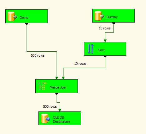
Figure 21: Running the SSIS package to verify the results
One other check we can do is to look at the data that has been inserted into the Merge_Output table. In SQL Server Management Studio (SSMS), run a SELECT statement that retrieves all rows from the Merge_Output table in the Demo database. The first dozen rows of your results should resemble Figure 22.
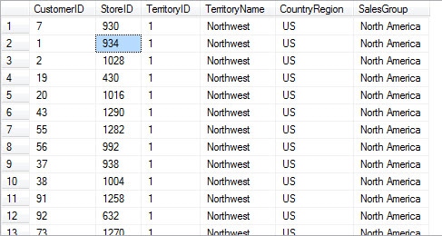
Figure 22: Partial results from retrieving the data in the Merge_Output table
Summary
In this article, we incorporated the Merge Join transformation into the data flow of an SSIS package in order to join data from two tables in different databases. We then created a third table based on the contents of the original two. In future articles, I hope to tackle error handling, deployment and many other tasks.
This document contains proprietary information and is protected by copyright law.
Copyright © 2026 Red Gate Software Limited. All rights reserved
Load comments