I once worked at a large financial institution where we had a policy in place that went …

“All procedures that are to be promoted must have their execution plan and STATISTICS IO data attached with the promote form, for review by DBA group”.

 A policy that, at first, might seem an intolerable imposition turned out to be a great habit to foster. We, the DBA group, could easily identify poorly performing queries, make notes and return it to the developers for them to modify.   The developers soon realized that they learned better techniques over time by studying the execution plans and STATISTICS IO data;  

In this article, I’d like to pass on what I learned about these two simple sources of information from SQL Server, because they are specifically designed to assist the developer to speed up the performance of queries:

You need the outputs from both together to make best use of them. In this article, I’ll take a real example of a large SQL query to illustrate how they will help solve the puzzle, and, hopefully, provide a nice clear picture rather than the jumbled puzzle pieces.

STATISTICS IO provides detailed information about the impact that your query has on SQL Server.  It tells you the number of logical reads (including LOB), physical reads (including read-ahead and LOB), and how many times a table was scanned.  This information helps you to establish whether or not the choices made by the optimizer are as efficient as possible at the time. 

This is powerful information to have when used together with the Execution plan.  Sometimes, for example, you’ll run a query and find that the Execution plan displays an index being used, yet STATISTICS IO shows that the index is doing 10 million logical reads.  At that point, you can re-evaluate the index choice and make sure there is no better way to write the query to use a more efficient index (less IOs).  The ideal solution is to use the least number of logical reads to perform your operation.  The fewer the logical reads, the faster the response and the lesser the impact on the Server.

Lesson 1: Breakdown of ‘STATISTICS IO’

STATISTICS IO can be set as an option when you execute a query. A message is sent via the connection that made a query , telling you the cost of the query in terms of the actual number of physical reads from  the disk and logical reads from memory, by the query. In SQL Server Management Studio, it will appear with the result of the query in the results pane  (under the messages tab, if you are using the grid)

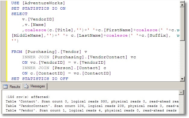
STATISTICS IO helps you to understand how your query performed by telling you what actually happened.  This shows you the IO that was incurred for each object, including the number of times it read a given object, the amount of logical/physical IO, and the order of access. 

What Statistics IO means

I took a single line from the output of STATISTICS IO and it is shown below.  We will take each phrase in the order in which they appear from left to right, though this is not necessarily the order that you will concentrate on, once you begin your tuning.  I’ll explain that later. 

Scan count (208,450)

This number tells us that the optimizer has chosen a plan that caused this object to be read repeatedly    This number is used as a gauge later on in the process and you will see what object it is being scanned when I go over the execution plan. This number does not change unless you alter the query.

Logical Reads (716751)

This number tells us the actual number of pages read from the data cache.   This is the number to focus on because it does not change unless you change the actual query structure or index structures.  Most common changes are the joins within the WHERE clause, parameter values, or  index structures.

Physical Reads (1421)

This is the number of pages actually read from the disk.  These are the pages that weren’t already in cache and so it is an interesting figure to monitor as it has a direct effect on the performance of the query.  SQL Server does all of its work within its caches.  If there is a requested page that is not in cache, it will read it from disk and place it in cache, then use that page.  If you were to run your query multiple times in a row, you would see your physical reads decrease and ultimately become 0 (so long as there is enough room in memory to store all of the pages required).  Because the physical reads change based upon memory pressure and not query design, I tend to ignore this figure.

Read-Ahead Reads (996)

This number tells us how many of the physical reads were satisfied by SQL Servers ‘Read-ahead’ mechanism.  This is directly tied to physical reads, so if there are no physical reads, you will have 0 for Read-Ahead reads.  I ignore this just like I ignore the Physical Reads.  This number will fluctuate as pages are swapped in/out of memory.   Although this is considered a type of physical read and whether or not SQL Server will do a physical read is based upon if the page exists in memory or not, index fragmentation will affect this number.

LOB Logical Reads (0)

We are not reading in any Large Objects (text, ntext, image, varchar(max), nvarchar(max) and varbinary(max)) in this particular example so this number will be 0.    The query used later on in this document does not request any Large Objects so this number is 0.  Should the query you are tuning at the time request large objects, you will see this number grow.  Pay attention to this number, just like the Logical Reads show above.

LOB Physical Reads (0)

This is the number of physical reads the server performed to fetch the necessary pages to satisfy the query.  Again, being physical we have no control over this.  Ignore it.

LOB Read-Ahead Reads (0)

This represents the number of physical reads satisfied by the Read-Ahead mechanism.  Nothing you can affect, without tuning the physical server, nothing to look to tune.

The STATISTICS IO Output

Here is part of a real query that I’ve chosen because it represents the reality of what has to be tackled in the working day of a DBA or developer. The real query is over 700 lines long so I’ll just show the tail of the query from the ‘JOIN’ clause onwards.

.  Listed below is the actual output of the STATISTICS IO request from executing this query..

Key Items of STATISTICS IO

Now that we have gone over each item that the STATISTICS IO provides, we’ll home in on what I call the key items, those that you can effect by  tuning your query.  The items are the scan count and the  logical reads.  I use these numbers in conjunction with the Execution plan output.  Now that you understand what each item within the STATISTICS IO output represents, I will now dig into the Execution plan of the above query.  You might be thinking to yourself “Why do that now?  We just started with the STATISTICS IO part”.  The answer is that you cannot properly alter any of the key items  (scan count and logical IO) without an understanding of Execution plans.  You need to use both outputs together.

Lesson 2: Execution plan Dissection

Now it’s time to take a Execution plan apart.  This will be your most important guide for identifying and fixing problem queries  You will begin to see the how you can affect the figures being returned by STATISTICS IO if you determine the best index and join usage .  Here is the Execution plan that corresponds to the STATISTICS IO output shown above.  To properly fit onto the page it’s hard to see the individual components.  Click on it to see it full-size  Since the output of the Execution plan is too large to display clearly on the page, I will break it into individual sections.

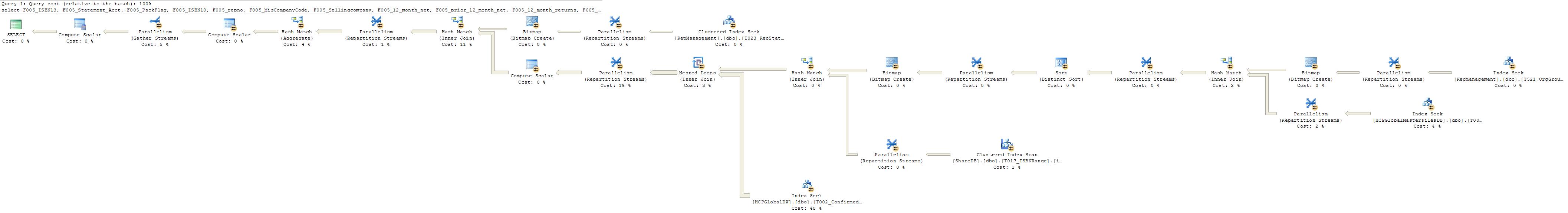
Start with the right-most top piece, since the end result of the Execution plan will be on the left. 

There are two things that you ought to keep in mind when you start inspecting the output. You will want to check the main access points (table scan, index scan, index seek, type of index) and the little % below each step.  All steps must add up to 100% and you will find, as you reduce one step, then another step will surely increase.  It’s the nature of the beast and you just want to make each step as efficient as you can

Taking a look at the execution fragment above, you will see that we are accessing two tables via an index seek. This is a more efficient way  to use an index than an index scan. The execution plan output  gives you the fully-qualified ‘database.owner.object.index’ syntax for each object.  If you mouse-over one of the images you will see something like this:

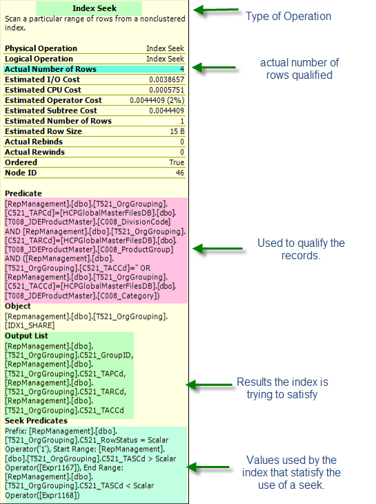
This gives a great deal of information about how SQL Server is accessing that index, and about what it is expecting to retrieve.  If you are stumped as to the reason why an index might be scanning  instead of seeking, or why SQL Server is doing a table scan instead of using an index, this is where you go.

Let’s take a moment to dissect the information presented by the image above using the highlighted sections as guides..  The first piece of information is the type of index access, which in this case is a seek.  This means that SQL Server knows exactly where to start looking for the information within the index;  much the same way if you were looking up my last name in the telephone book.  You could go straight to ‘Richberg’ and then look at each listing until you found ‘Josef’. 

The next highlighted section is Actual Number of Rows, which is exactly as it sounds.  SQL Server found 4 records that match all of the criteria given  I find this very useful when trying to determine how effective a given index is or specific criteria are  The Predicate section is next.  This shows you the all the pieces this index uses to qualify a row.  It will show you any known values, value ranges, and joins to other tables (and on what columns).  You will see this on an Index Seek and an Index Scan.  This is an area I use to help determine if you index is being use as effectively as possibly. 

You might look at this and notice ‘I am missing a join to table X’ or ‘I shouldn’t be joining to table y’.  You may not see this section at all.  That would mean the index is being scanned in its entirety and there are no criteria to restrict the rows at this point.  The Output List shows you what columns the index will be returning.  If the index can satisfy all of the columns requested, it is considered a ‘Covered’ index, otherwise the index will need to get the additional columns from the underlying structure (clustered index if it exists or the table).   The final section is Seek Predicates, which shows the actual columns, values, and criteria (<,>,=) used to satisfy the seek.  If this where an Index Scan you would not see the Seek Predicates section. I can tell by reading this section, I am looking for C521_RowStatus='1' and C521_TASCD > [Expr1167] and C521_TASCD<[Expr1168].  I would have to go back to the query to see what the actual values of [Expr1167] and [Expr1168] are, but I would know where to look, because it would be near > and <.   . 

Understanding how and why SQL Server determines particular paths between objects to satisfy your query and ultimately provide your data, you can tune your queries and database structures to be more efficient in their use of resources, which is the ultimate goal in tuning.

The next set of objects is below.

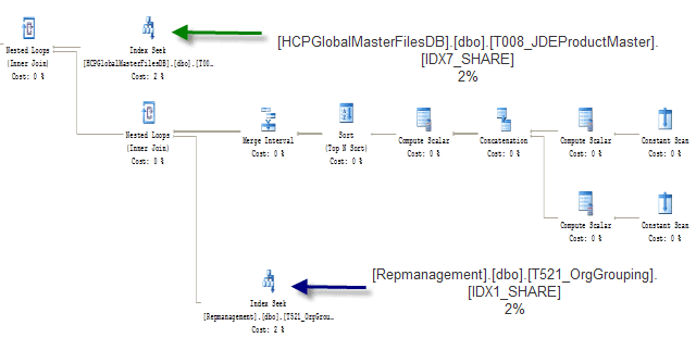
Here you can see that  T017_ISBNRange is accessed via a clustered index seek and that T002_ConfirmedSalesDetail is access via a non-clustered index seek.  They are joined together by a Nested Loop.  The output of that is then joined to the output of the non-clustered index seek of T023_RepStatementI would like you to take note as we walk through the graphical execution plan how each step from the right connects to objects on the left and each object from the bottom connects upwards towards the top.  The sequence logically moves from left to right, bottom to top and eventually towards, in this case a select.  Continuing, the output of all 3 indexes is joined again to a non-clustered index seek on T008_JDEProductMaster.  This is shown in the image below.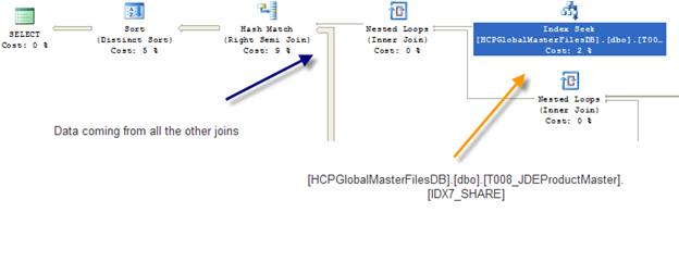

 We are now at the end of the diagram.  A nested loop is used to join the result coming from T008_JDEProductMaster and that of the nested loop below it, shown by the orange arrow.  The result of that output is joined with the results of other operations below, shown by the fatter line pointed to by the blue arrow.   A final hash match is used, taking up 9% of the total cost, then Sort (I have a few group bys in the query creating the need for a sort) and then the Select, which is the result, being sent back to the calling application.  Another piece of useful information can be gleaned by clicking on the lines between each set.

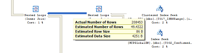
This information tells me that there are 208,453 qualifying rows that are the result of joining T017_ISBNRange and T002_ConfirmedSalesDetail.  If there is a significant difference between the estimated and actual figures, check the statistics of your indexes as they might be stale.  The other pieces of information, estimated row size and estimated data size can only be modified if you adjust your join columns or select statement.    

Lession 3: Into the Wild Blue Yonder (Real World Example)

I am going to switch up gears a little bit to show you how you can

• use the Execution plan output to determine what changes to make

• use your STATISTICS IO output to make sure that change was correct. 

On rare occasions you will find  that a query strategy that looks sensible in the S proves to be poor in the IO department, making you scratch your head and re-think your choices.  I find this situation most often is the use of an in ‘incorrect’ index.  You might be asking yourself, ‘How can an index be incorrect’?   Let’s look at the images below and use those as examples to better explain.  .

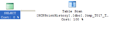
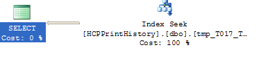
The above query produces the following execution plan and STATISTICS IO output.

 

The optimizer is looking for the most efficient path to obtain your information.  The first choice it has is to go directly to the table for the information, which requires a table scan.   A table with no index is akin to a book with no index.  If I asked you to find me the pumpkin pie recipe in the ‘Great Recipe Book’, but the publisher left out the index, you would have to start at the first page and leaf through each and every page until you found it.  You would most likely have to leaf through the whole book, since you won’t know if there is more than one recipe.

Scanning through our ‘recipe book (T017_TradeReceiving)’ required 4,661 logical reads.  While it only took 1 second ,you want to keep in mind the fewer resources  used by each and every query, the overall better performance you will get out of your entire system.  Knowing this is a table scan, you want to try to see if you can put some index on this which will reduce the effort it takes SQL Server to retrieve the data you want.

We decide to call the editor and say ‘This book needs an index of some sort’.  The editor agrees and publishes a new book with an index on categories.  Now when you go to look up pumpkin pie, you go to the back and look at ‘pies pgs 120-155’. This index is more efficient, but you still have work to do, you have to look at 35 pages. 

Continuing this example going forward, we decide to put an index on the  column ‘C017_DateLastReceived’. 

The syntax for creating the index is:

You can see that the query produces a table scan, which results in 4,663 logical reads.  There is no physical IO so the time we get (1 sec) is ‘as good as it gets ‘ for this query.  The first thing that comes to mind is that there may not be an index on C017_DateLastRecived.  It turns out that there isn’t one, so I will put one on the table

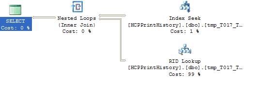
Just as in the cookbook example above, were you decide to use the index to retrieve your pie information, the optimizer has decided to use the index to retrieve the data instead of doing a table scan.  The output of the execution plan gives insight into the new path.  The output of the STATISTICS IO verifies that it is a better path by showing a reduction in logical reads.

We are now down to 120 logical reads, a significant improvement over the original 4,663, but in looking at the graphical execution plan,   I can see there is additional work being done.  The RID Lookup tells me that SQL Server needs more information than is being supplied by the index.  Back to our cookbook example, even though the index tells you the exact pages to go for pie recipes, you must go back into the cookbook to read the actual pumpkin pie recipe.  To find out what is missing in our real world example we need to highlight the RID Lookup image and our pop-up looks like this:

 If you look at the highlighted section, you will see the missing columns, C017_SecondItemNumber and C017_ThirdItemNumber.  This tells me we can improve this one step further.  Back to our cookbook example.

You have cooked so many pies by now, you don’t need the instructions on how to cook a pumpkin pie, you just want an ingredients list.  You contact the editor again and say ‘Can you add an ingredients list for each recipe?’.  The editor takes your suggestion and sends you the new book.  Now when you go the new new ‘recipie appendix’, you look up pumpkin pie and see all the ingredients right there.  You don’t have to go back to page xxx to find them.  This is optimal.  Let’s do the same thing with out table.

Let’s modify the index to provide the necessary information.  Here is the statement to drop the current index:

We will recreate the index to include the missing columns.  We will be using the syntax for creating an index with ‘included columns’, which is available in SQL Server 2005 or greater.

You will notice the keyword ‘included columns’.  This is a new space saving  feature in SQL Server 2005 and higher.  The columns listed in the include section can only be used to satisfy columns requested in the select clause of your SQL statement, not the WHERE clause.  This is because the included columns  are created in the leaf of the index and not the intermediate levels.  This means the optimizer has no path to them.  In the cookbook example, I cannot use an ingredient to find a recipe.

In SQL Server 2000, the columns in an index existed at all levels (root, intermediate, leaf) taking up much more space than needed.

If you are using SQL Server 2000, your create index statement would be:

After creating the new index we re-run the select statement and find the following output from execution plan and STATISTICS IO.

 

Modifying the non-clustered index to include those two columns reduced the logical reads to 4, a reduction in resource use by over 1000%.  You might be asking, ‘Why didn’t you use a clustered index?’  The answer is simple:  I example I was looking to illustrate was just because an index is show as being using in the graphical execution plan, doesn’t mean there I no tuning to be done.  I wanted to show you the progression from a table with no indexes, to a table with a moderately efficient index, to a table with a very efficient index and the path to get there.  A clustered index is by it’s very nature  is ‘covered’ and would have left out the 2nd step.

You will have seen that your query has used over 1000 times less resources just by improving the access through an index  and thereby reducing your final reads to  4. 

Conclusion

While you have cut your time from 1 sec to 0 seconds which seems negligible, you have achieved  a dramatic reduction in the load on the server. Queries must return data as fast as possible, but must use resources efficiently too.  If each query is designed to be as resource efficient as possible your sever will be able to do more, in a shorter period of time, with less.  Consider SQL Server a community where every query  has an impact, either direct or indirect on the all the other queries running.  Having a single poorly performing query can affect any number of optimized queries, since they are reside in the same SQL Server.  They share the same resource pool (memory, disk, CPU, etc).  Having a poorly designed query take millions of more reads than it needs, puts  undue pressure on the I/O subsystem and the cache, which has a trickling-down effect on the other queries, which results in the entire server looking ‘slow’..

I hope this article will lead to the production DBAs getting calls at 3 am about performance issues and then for them to have to use some of the complicated DMVs to find those slow  queries.  Tuning your queries properly, prior to their introduction into production is a much better practice, than looking to correct the problem after the application goes live.