
It has been about 4 years since Brent Ozar posted his famous blog post on collecting performance counters. This information turned out to be extremely useful for both accidental and professional DBAs. About 4 years later I ran into Jonathan Allen’s article (Getting baseline and performance stats – the easy way.), which is an upgrade to Brent’s blog. Jonathan offers a slightly more sophisticated way of running the Perfmon process from a command line. By appending the proper parameters, this method does speed things up.
In this article, I would like to build on what Brent and Jonathan have written to propose an even more flexible method for SQL Server performance data collection.
typeperf.exe: Command-line performance-data collection
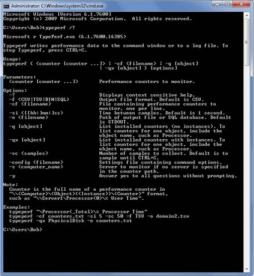
As Jonathan Allen mentions in his blog, typeperf.exe is a powerful command. Here is a screenshot of all parameters the command accepts and their short description (as the output of ‘typeperf.exe /?‘ would show them):
As we can see, there are several options which allow us to save the output of the typeperf in different formats: CSV, TSV, BIN, SQL. (CSV = Comma Separated file, TSV = Tab Separated file, BIN = Binary file, SQL = SQL Server table)
And here is the moment when I start thinking about my preferred choice of format.
As a DBA, I do not like CSV much, unless I really need to export some trivial data and email it to someone. With CSV there is also a security risk, since it is nothing but a text file saved on the file system; same goes for the TSV and the BIN formats.
Furthermore, the processing times are significant, since it is a two-step process: first we would have to wait for the counters to collect into the file, and then we would have to open them and manipulate the data so that we extract what interests us.
Now, wouldn’t it be great if we could have the performance data collected directly into our already secured SQL Server? (I talk about security because I can personally think of at least a few scenarios where even performance data in the wrong hands can cause a lot of trouble.)
Furthermore, if we could import our performance counters to SQL Server database, that would mean that we can query the data any time and we can write reusable code for the queries which will help us easily analyze data over and over again. It will also help us detect events, patterns, send notifications, if we wanted.
So, to get back on track: my choice for the performance data collection output is SQL.
How to collect performance data directly to SQL Server:
First, of course we need to set up a database which will contain our performance data.
For this exercise we will create a new database called ‘PerfmonCollector‘ by using the following script:
|
1 2 3 4 5 |
CREATE DATABASE [PerfmonCollector] ON PRIMARY ( NAME = N'PerfmonCollector', FILENAME = N'C:\Program Files\Microsoft SQL Server\MSSQL10.MSSQLSERVER\MSSQL\DATA\PerfmonCollector.mdf' , SIZE = 51200KB , FILEGROWTH = 10240KB ) LOG ON ( NAME = N'PerfmonCollector_log', FILENAME = N'C:\Program Files\Microsoft SQL Server\MSSQL10.MSSQLSERVER\MSSQL\DATA\PerfmonCollector_log.ldf' , SIZE = 1024KB , FILEGROWTH = 10%) GO |
Second we would need to connect Typeperf to SQL Server. Let’s run the ODBC Data Source Administrator (we can access it by clicking Run… and then ‘odbcad32.exe’).
The following screen will be presented:
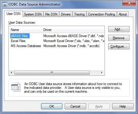
In the tabs of the administrator we see ‘User DSN’ and ‘System DSN’. The difference is that the User DSN is visible only to the current user, and the System DSN is visible to all users of the machine, including the NT services.
So, let’s choose a ‘User DSN’, since we do not want anyone but us to access our database. Let’s create it:
1. Click Add… button and select SQL Server driver type
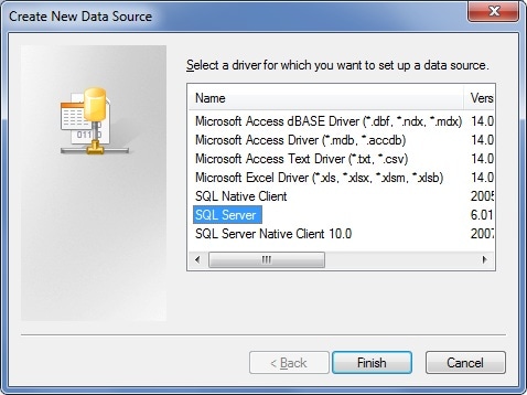
2. Click ‘Finish’. A Data Source wizard screen will show up:
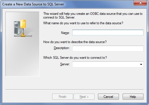
3. Fill in the name of the Data Source and the SQL Server instance name. In my case, I would go for ‘SQLServerDS’ and (local).
4. In the next screen we would have to provide the login details:
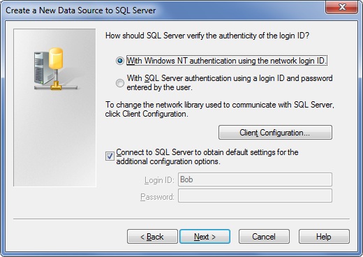
I will use Windows authentication. Click next.
5. In this screen it is important to select our ‘PerfmonCollector‘ database:
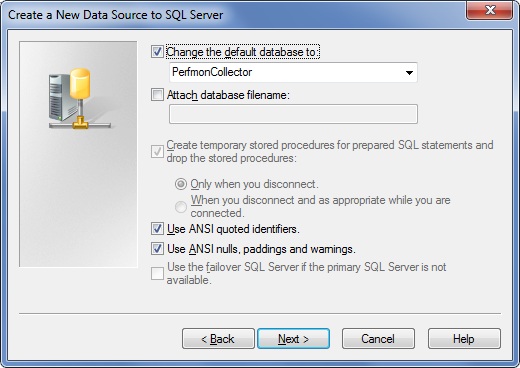
Click Next.
6. In this screen we would leave the settings as default:
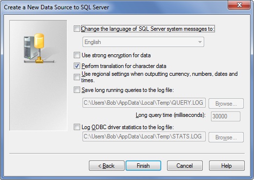
Click Finish.
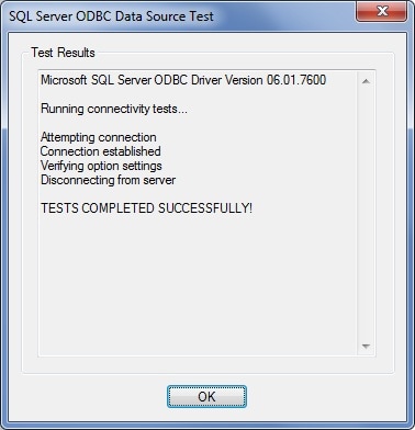
7. In this screen you will be presented with an overview of the settings and with a chance to test our connection.
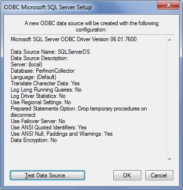
Click the ‘Test Data Source…’ and make sure that the test is successful.
Now that we have a database and a connection, the next step is to gather some counters and to save the results into our database.
Collecting the counters:
Let’s say that we want to collect the values from the counters mentioned in Jonathan Allen’s blog post:
- Memory – Available MBytes
- Paging File – % Usage
- Physical Disk – % Disk Time
- Physical Disk – Avg. Disk Queue Length
- Physical Disk – Avg. Disk sec/Read
- Physical Disk – Avg. Disk sec/Write
- Physical Disk – Disk Reads/sec
- Physical Disk – Disk Writes/sec
- Processor – % Processor Time
- SQLServer:Buffer Manager – Buffer cache hit ratio
- SQLServer:Buffer Manager – Page life expectancy
- SQLServer:General Statistics – User Connections
- SQLServer:Memory Manager – Memory Grants Pending
- System – Processor Queue Length
What we need to do is create a text file on our file system, which contains the counters we need to collect. Keep in mind that there are 2 kinds of counters – machine counters and SQL Server specific counters. So if we have only one default instance of SQL Server on a machine and we would like to collect the performance counters, our text file will look like this:
\Memory\Available MBytes
\Paging File(_Total)\% Usage
\PhysicalDisk(* *)\% Disk Time
\PhysicalDisk(* *)\Avg. Disk Queue Length
\PhysicalDisk(* *)\Avg. Disk sec/Read
\PhysicalDisk(* *)\Avg. Disk sec/Write
\PhysicalDisk(* *)\Disk Reads/sec
\PhysicalDisk(* *)\Disk Writes/sec
\Processor(*)\% Processor Time
\SQLServer:Buffer Manager\Buffer cache hit ratio
\SQLServer:Buffer Manager\Page life expectancy
\SQLServer:General Statistics\User Connections
\SQLServer:Memory Manager\Memory Grants Pending
\System\Processor Queue Length
It is a bit more complicated with the named instances of SQL Server. The text file containing the counters for a named instance would look like this:
\Memory\Available MBytes
\Paging File(_Total)\% Usage
\PhysicalDisk(* *)\% Disk Time
\PhysicalDisk(* *)\Avg. Disk Queue Length
\PhysicalDisk(* *)\Avg. Disk sec/Read
\PhysicalDisk(* *)\Avg. Disk sec/Write
\PhysicalDisk(* *)\Disk Reads/sec
\PhysicalDisk(* *)\Disk Writes/sec
\Processor(*)\% Processor Time
\MSSQL$InstanceName:Buffer Manager\Buffer cache hit ratio
\MSSQL$ InstanceName:Buffer Manager\Page life expectancy
\MSSQL$ InstanceName:General Statistics\User Connections
\MSSQL$ InstanceName:Memory Manager\Memory Grants Pending
\System\Processor Queue Length
As you can see, in the case of a named instance, we would have to manually edit the text file and input the name of the instance for which we need to collect counters.
Depending on how many servers we have and how many instances of SQL Server reside on one physical machine, we would group our text files accordingly.
Let’s say that we have one physical server and 4 SQL Server instances; in this case I would create one text file containing the counters for the physical server (including the counters for the default instance) and then create 3 more files containing only the named instances’ counters.
For this article, however, I would collect performance data only from my named instance (the name of my instance is ‘SQL2005’) and my server.
So, I will create a folder ‘CounterCollect’ in my C: drive, and in the folder I will place my ‘counters.txt’ file containing my list of counters as follows:
\Memory\Available MBytes
\Paging File(_Total)\% Usage
\PhysicalDisk(* *)\% Disk Time
\PhysicalDisk(* *)\Avg. Disk Queue Length
\PhysicalDisk(* *)\Avg. Disk sec/Read
\PhysicalDisk(* *)\Avg. Disk sec/Write
\PhysicalDisk(* *)\Disk Reads/sec
\PhysicalDisk(* *)\Disk Writes/sec
\Processor(*)\% Processor Time
\MSSQL$SQL2005:Buffer Manager\Buffer cache hit ratio
\MSSQL$ SQL2005:Buffer Manager\Page life expectancy
\MSSQL$ SQL2005:General Statistics\User Connections
\MSSQL$SQL2005:Memory Manager\Memory Grants Pending
\System\Processor Queue Length
And now comes the most interesting part: running the cmd command which will start our data collection:
|
1 |
TYPEPERF -f SQL -s ALF -cf "C:\CounterCollect\Counters.txt" -si 15 -o SQL:SQLServerDS!log1 -sc 4 |
Here is a short explanation of the parameters:
- ‘f’ is the output file format
- ‘s‘ is the server from which we would like to collect counters
- ‘cf’ is the path to the text file which contains the counters
- ‘si‘ is a sampling interval, in this case every 15 seconds
- ‘o’ is the path to the output file, or in this case it is specifying the DSN we created earlier
- ‘sc’ is how many samples to collect, in this case 4, which means that the process typeperf will run for 1 minute and will collect 4 samples.
As you notice, there is a '!log1' after the DSN name. This is a way to give a name to our performance data collection set. For example, instead of 'log1‘ we could put ‘beforeCodeRelease'.
Note: do not be surprised if your first sample is sometimes 0. This is how typeperf works. This is because typeperf is getting the delta (the value difference) between the sampled intervals.
The results:
Let’s look at our ‘PerfmonCollector’ database.
We can notice that there are 3 new tables in our database, which were created by the typeperf:
|
1 2 3 |
dbo.CounterData dbo.CounterDetails dbo.DisplayToID |
Here is how part of the CounterData table looks:
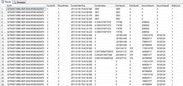
What do they contain? Here is some information from MSDN:
The CounterData table contains a row for each counter that is collected at a particular time. There will be a large number of these rows.
The CounterData table defines the following fields:
- GUID: GUID for this data set. Use this key to join with the
DisplayToIDtable. - CounterID: Identifies the counter. Use this key to join with the
CounterDetailstable. - RecordIndex: The sample index for a specific counter identifier and collection GUID. The value increases for each successive sample in this log file.
- CounterDateTime: The time the collection was started, in UTC time.
- CounterValue: The formatted value of the counter. This value may be zero for the first record if the counter requires two sample to compute a displayable value.
- FirstValueA: Combine this 32-bit value with the value of FirstValueB to create the FirstValue member of
PDH_RAW_COUNTER. FirstValueA contains the low order bits. - FirstValueB: Combine this 32-bit value with the value of FirstValueA to create the FirstValue member of PDH_RAW_COUNTER. FirstValueB contains the high order bits.
- SecondValueA: Combine this 32-bit value with the value of SecondValueB to create the SecondValue member of PDH_RAW_COUNTER. SecondValueA contains the low order bits.
- SecondValueB: Combine this 32-bit value with the value of SecondValueA to create the SecondValue member of PDH_RAW_COUNTER. SecondValueB contains the high order bits.
Information about the rest of the tables can be obtained from MSDN as well: DisplayToID ) ( and CounterDetails )
So, we have the data, let’s use it!
As I mentioned earlier, this method of collecting performance data is not only more secure than CSV+Excell, but also is more flexible. Remember, as we defined earlier our Perfmon collector command, we gave a name to our collector set. In this case we named it simply log1. For a real hands-on performance tuning sessions, though, we would like to name every set with its own meaningful name. (For example, let’s say that we would like to measure the server’s performance between 10am and 11am every day, when we are running a specific batch job.)
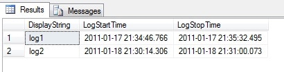
The name of the collector set is found in the DisplayToID table, in the DisplayString column. There we also see the LogStartTime and LogStopTime. The DisplayToID table is joined to the CounterData table by the GUID.
For my test case in this article I am using two data collector sets called log1 and log2. Both sets are using the same counters as mentioned above.
The first thing we would like to do is to verify how many different servers we have collected the data from. By running this query we can check:
|
1 2 3 |
SELECT DISTINCT [MachineName] FROM dbo.CounterDetails |
In my case I would get only one server: \\ALF.
Now let’s check what data collection sets we have and what their start and end times are:
|
1 2 3 4 |
SELECT [DisplayString] , [LogStartTime] , [LogStopTime] FROM dbo.DisplayToID |
Here is the result:
Now let’s check the values we have collected for a specific counter for a specific server:
|
1 2 3 4 5 6 7 8 9 10 11 12 13 14 |
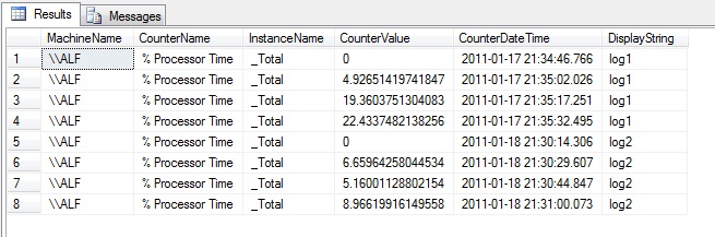
SELECT MachineName , CounterName , InstanceName , CounterValue , CounterDateTime , DisplayString FROM dbo.CounterDetails cdt INNER JOIN dbo.CounterData cd ON cdt.CounterID = cd.CounterID INNER JOIN DisplayToID d ON d.GUID = cd.GUID WHERE MachineName = '\\ALF' AND ObjectName = 'Processor' AND cdt.CounterName = '% Processor Time' AND cdt.InstanceName = '_Total' ORDER BY CounterDateTime |
This query will return the Processor Total % utilization time as well as the counter collection time and the collector set name. Feel free to use this query as a template for exploring other counters as well.
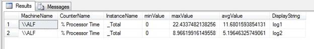
And here is one more query which will give some aggregations:
|
1 2 3 4 5 6 7 8 9 10 11 12 13 14 15 16 17 18 |
SELECT MachineName , CounterName , InstanceName , MIN(CounterValue) AS minValue , MAX(CounterValue) AS maxValue , AVG(CounterValue) AS avgValue , DisplayString FROM dbo.CounterDetails cdt INNER JOIN dbo.CounterData cd ON cdt.CounterID = cd.CounterID INNER JOIN dbo.DisplayToID d ON d.GUID = cd.GUID WHERE MachineName = '\\ALF' AND ObjectName = 'Processor' AND cdt.CounterName = '% Processor Time' AND cdt.InstanceName = '_Total' GROUP BY MachineName , CounterName , InstanceName , DisplayString |
Here is the result and as you can see it is quite easy to compare the two data collector sets.
From this point on, I am sure that any DBA would be able to easily write queries and find out performance events, patterns and tendencies.
Summary:
In this article I describe a flexible and secure method for collecting data from the collection of performance counters from servers and SQL Server instances. This method avoids the limitations of Excel spreadsheets, and brings great possibilities to the DBA to query the data directly, so as to home in on the cause of performance problems (or the lack of them, hopefully!) in the monitored systems.
This document contains proprietary information and is protected by copyright law.
Copyright © 2026 Red Gate Software Limited. All rights reserved
Load comments