Gaps and islands analysis supplies a mechanism to group data organically in ways that a standard GROUP BY cannot provide. Once we know how to perform an analysis and group data into islands, we can extend this into the realm of real data.

For all code examples in this article, we will use a set of baseball data that I’ve created and maintained over the years. This data is ideal for analytics as it is large and contains data quality that varies between very accurate and very sloppy. As a result, we are forced to consider data quality in our work, as well as scrutinize boundary conditions for correctness. This data will be used without much introduction as we will only reference two tables, and each is relatively straightforward.

Once introduced, we can obtain metrics that may seem challenging to crunch normally, but by using a familiar and reusable gaps/islands algorithm, we can make it (almost) as easy as cut & paste.

Gaps and Islands: Definitions and Data Intro

Our first task is to define a programmatic way to locate gaps and islands within any set of data. To do so, consider what a boundary is within different data types:

• For a sequence of integers, a boundary can surround missing values.
• For dates/times, a boundary can represent the start or end of a sequence of frequent events that are chronologically close together.
• For decimals, boundaries may be defined by values that are within a small range of each other.
• For strings, missing letters or letter sequences may define a boundary.

These represent a starting point for considering ways to slice up data. A critical aspect of this work is that the result set of gaps/islands analysis will vary in size. For example, if we wanted to measure the number of winning streaks by a sports team as a data island, then there could be any number from zero to (N + 1) / 2 islands, given a set of N rows. This assumes a repeating sequence of winning and losing “streaks” of one game each.

The following diagram shows a set of 10 win/loss events and different ways that islands of data could look:

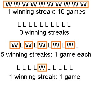
The image illustrates result sets of 0, 1, and 5 rows for island counts. Note that a single winning streak of 1 game and a single winning streak of 10 games each result in a single identifiable island of data. The key here is that if we are generating a dataset of winning streaks, the result set will vary in size based on the underlying data.

Let’s jump into baseball data and crunch winning streaks as islands of wins and losing streaks as islands of losses. Conceptually, islands are easier to manage and understand than gaps. This convention also allows us to write all our queries similarly, regardless of the results we are seeking.

Here is a sample of the data we will be working with:

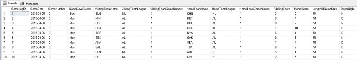
The results show a row per game with a sample of metrics, including team names (abbreviations), game date, score, and more. GameNumber indicates if a game was part of a double-header so that we know the order of games within a given day, when applicable. The details continue for many more columns and tell us who played each position, the umpires, and totals for many metrics within the game. For the sake of our work, the most basic high-level details are all we will need.

We will use an additional table that contains play-by-play details for each game. The following is a sample of that detail:

This table contains a row per play per game. A play is usually an at-bat, but may also consist of an error, stolen base, or other action that can be taken during a game. A single game could have over a hundred events associated with it. Like GameLog, the detail can get exhaustive, but we will focus on high-level, easy-to-understand metrics.

This data contains 219,832 games spanning from 1871 through 2018. There is a total of 12,507,920 events associated with those games. With the data introduced, let’s define a winning streak as a set of wins bounded by losses or ties. With that simple definition in mind, we can dive in and crunch our data.

Gaps and Islands: Calculating Streaks

The simplest analysis we can perform is to determine winning and losing streaks. From a data perspective, streaks can be described as islands of wins or losses. To code this, we need to formulate a reliable and repeatable process so that we are not writing new code over and over for each query. The following steps through what we need to accomplish to complete this analysis.

1. Gather a dataset

No metrics can be crunched without a candidate dataset that provides everything we want without noise or distractions. For baseball data, we will be creating a set of games. For example, if we wanted to find regular-season winning streaks for the New York Yankees, we would need to pull every regular-season game that they played in:

Here, we filter on any game where the home team or away team was the Yankees (NYA). We then filter to include only regular-season games (REG). GameLogId is an identity primary key and is used to ensure each row is unique and ordered chronologically.

Lastly, we compare the home and away scores to determine if the game was a win, loss or tie as follows:

• If the Yankees are the home team and the home score is greater than the visiting score, then it is a win.
• If the Yankees are the visiting team and the visiting score is greater than the home score, then it is a win.
• If the Yankees are the home team and the home score is less than the visiting score, then it is a loss.
• If the Yankees are the visiting team and the visiting score is less than the home score, then it is a loss.
• If the scores are the same, then it is a tie. This is uncommon but has happened enough times to be statistically significant.

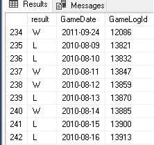
The results are a narrow dataset that lists every game the Yankees have ever played, as well as the result:

2. Determine the Start and End of Streaks

We now want to look at the data above and identify the dates that every winning streak began and ended. To do this, we need insight into the next and previous games. A winning streak begins when a win is preceded by a game that is not a win. A winning streak ends when a win is followed by a game that is not a win.

The easiest way to accomplish this is to use LEAD and LAG on each game to return whether the previous and next games were wins, losses, or ties:

Note that the contents of the result field are copied verbatim into a LEAD and LAG statement. Each are ordered by the game date and ID columns, ensuring chronological order and no chance of ties. Window functions operate over a window (set of rows) and here we are defining the window as the entire dataset with this particular ordering.

In addition, a column was added with a ROW_NUMBER, which numbers every game in order. This allows for some additional math later, such as streak length:

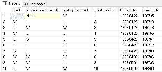
Note that the previous game result is NULL for the first row. Similarly, the next game result will be NULL for the last row in the dataset.

With this work out of the way, we can now identify the start and end of streaks. A critically important mathematical note on this data is that the number of starting and ending data points will always be equal. If we find 100 winning streaks, we know that there will be 100 starting points, 100 ending points, and all 100 of each can join together in order to provide a full dataset.

To find the beginning and end of each streak, we will encapsulate the code above in a CTE and query it accordingly:

This code is starting to get lengthy, but it’s building on the TSQL we have already completed. CTE_ISLAND_START returns the date and location for the start of a winning streak, and CTE_ISLAND_END returns the date and location for the end of the winning streak. We add in a new ROW_NUMBER to ensure we have island numbers that fully describe the logic presented above. Note that we check for NULL to ensure that we identify the start and end of the dataset as legitimate boundaries.

3. Join Streak Start and End Dates and Return Results

Our final task is to join the beginning and end of each streak together to generate a dataset we can report from:

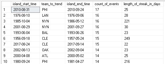
Note that all we have added here is a final select that joins together our CTEs on streak number (the island_number column). As a bonus, we can subtract island locations and find the difference between the start and end dates to determine how long a streak was, both in days and games. Ordering by streak length in games allows us to view the longest streaks first:

The results are straightforward and tell us the longest winning streaks of all time for a single team. Measuring losing streaks, tie streaks, or any other metric as a streak would only require changing the results that we define in the first CTE and then join on and filter in subsequent CTEs.

The syntax above seems lengthy, but now that it is defined, we can reuse it for all of our additional examples. We can customize and return a variety of more complicated insights without changing much about this code, making it a nice way to solve these analytic questions.

Using PARTITION BY to Calculate Streaks Across Multiple Entities

Analyzing winning streaks for a single team is useful, but what would be more interesting would be to look at a single team versus all other teams, or all teams versus all teams. This would provide an overall view of winning streaks, regardless of the opposition.

If we wanted to know the longest winning streaks by the Yankees versus other individual teams, we could accomplish that task by the use of PARTITION BY in all of our window functions. By partitioning by the opposing team, we can generate a list of winning streaks that are broken down into subsets for each team. With that single change, we can get a completely new set of results:

Note that all window functions now include a PARTITION BY that operates on the opposing team. Window functions operate over a window, and here we are defining the window as a dataset per team. This means that we will have a window per team, rather than a single window for all teams.

For the GAME_LOG CTE, this calculation requires partitioning by a CASE statement that is similar to how we determined if a game was a win or loss. In the remaining CTEs, we can use the opposing_team column to more quickly generate these results (and with less code). Also, note the following:

The final SELECT is nearly identical to all previous demos.

CTE_ISLAND_START and CTE_ISLAND_END are identical to previous demos except in the use of PARTITION BY to further subdivide the dataset.

These similarities allow us to reuse the same syntax repeatedly with a high level of confidence in the results:

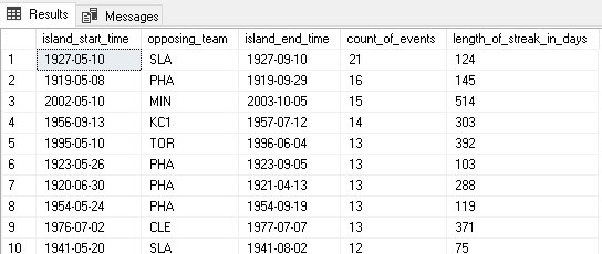
The results quickly tell us the longest winning streaks the Yankees have had versus all other teams in the regular season, with the St. Louis Browns being on the historical losing end of this dataset.

The dataset is interesting, but it begs the question: “How do we calculate winning streaks by all teams versus all teams?”. If we would like to see all winning streaks, regardless of team, then we will need to further customize our queries above as follows:

1. Include both home and visiting teams in all queries.

The GAME_LOG CTE needs to be adjusted with a UNION ALL to ensure that we get all games from the perspective of the home and away teams. In other words, we need to double the size of this CTE to ensure that we have a row per team per game.

1. This change will necessitate a separate CTE to appropriately order the dataset for further analysis.
2. Instead of partitioning by the opposing team, we need to partition by both the team to trend and the opposing team. This will generate a much larger set of windows to analyze.

The following is the final result of the changes above:

While the changes are readily apparent, the code overall is very similar to what we wrote earlier. Window functions operate over a window, and here we are defining the window as a dataset per each pair of teams. This means that we will have a window for every set of teams that have played each other. This is a far larger number of windows than earlier but is necessary to be able to calculate streaks in aggregate across all possible matchups. The results are as follows:

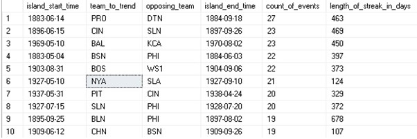
We can observe that the top winning streak for the Yankees is only number 6 on this list with the top 10 streaks ranging anywhere from 1883 to 1970. Streak lengths are often quite long as many spanned multiple seasons.

Longest Winning Streaks for Any Team

Another similar problem we may wish to solve is to determine the longest overall winning streaks for all teams in baseball. Earlier we calculated this metric for a single team, but there is value in being able to do so for all teams in a single query.

Fortunately, we have already done much of the work on this (and then some). To find the longest winning streaks for all teams in aggregate (not versus any specific team), all we need to do is remove the opposing team from all PARTITION BY clauses. The remaining TSQL remains nearly identical:

Window functions operate over a window and here we are defining the window as a dataset per team. This means that we will have a single window for every team that has ever won a game. This contrasts our previous query, which generated far more windows to perform analysis over.

The results are as follows:

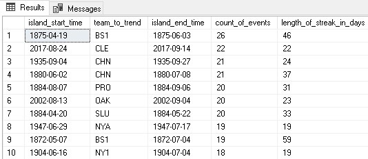
We can see that the longest winning streak of all time was accomplished by the Boston Red Stockings in 1875.

Note that the results do not include ties. Adjusting our work to include ties would require that we:

1. Change CTE_ISLAND_START and CTE_ISLAND_END to consider a streak start/end bounded by a loss, and not a loss or tie.
2. Adjust the count of events to exclude ties. This avoids reporting a streak that was more games won than were actually won.

Alternatively, we could count a tie as a win for record-keeping. This would simplify the T-SQL but report occasionally inaccurate data. For these metrics, adding a notes or has_ties column would better allow us to denote if a tie occurred.

The simplest approach would be to omit ties altogether and pretend they do not exist, like this:

This code explicitly filters out ties, so the end results will completely ignore them. We get no insight into whether a streak included ties but could easily join our result set back into the underlying data to gather that information, if it were important.

Filtering Results to Answer Obscure Questions

When observing any data analysis long enough, we are eventually surprised by obscure data requests or facts that might not come naturally to us. In sports, like in business, people are looking for new knowledge that can provide any statistical benefit. Does a player perform better at night? How about in the cold? Does being right or left-handed matter?

Statistics across these metrics sound mind-bogglingly complex but are incredibly easy to crunch using code we have already written. The key is to alter the filter of our primary dataset. The remainder of the gaps/islands analysis can be left as-is and will perform exactly as we want.

For example, imagine we wanted to track winning streaks for all teams at night. The T-SQL to make this happen is as follows:

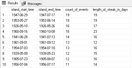
The only change is that we added a filter to each part of the UNION dataset to filter out all games that are not night games. We check for NULL as some older games have no record of time of day. The results are as follows:

The results provide some obscure, but interesting data. Oftentimes, scenarios like these will seem nonsensical until a real-world scenario arises where they make perfect sense. For many statistical analyses, being able to improve predictions even by a small percentage can have a profound impact. For job functions such as sales or marketing, timing questions arise often and knowing the optimal ways in which to engage people can be the difference between success and failure.

Conclusion

The TSQL introduced in this article was not for the faint of heart. Breaking it into smaller pieces and viewing each chunk as a logical step towards getting our result set helped make it easier to read and understand. To summarize, the general process used in every islands/streaks analysis:

1. Create a dataset with a definitive win/loss definition.
2. Order the dataset so that each event can be numbered.
3. Generate a list of island starting points
4. Generate a list of island ending points
5. Join the starting and ending points together and return results.

Once this syntax is established, every query will be similar to the rest of the queries we write. Copying, pasting, and modifying this TSQL to create new filters, partitions, or metrics is recommended as a far faster and reliable alternative than rewriting this code repeatedly.

Using this style of analysis, we can crunch vast amounts of data into meaningful groups that can measure success and report on how events relate to other nearby events. While other tools such as Python or R can be used to crunch this data in a similar fashion, being closer to the data allows for easier customization and more reliable control over performance.