Clustered indexes are the cornerstone of good database design. A poorly-chosen clustered index doesn’t just lead to high execution times; it has a ‘waterfall effect’ on the entire system, causing wasted disk space, poor IO, heavy fragmentation, and more.

This article will present all the attributes that I believe make up an efficient clustered index key, which are:

• Narrow – as narrow as possible, in terms of the number of bytes it stores
• Unique – to avoid the need for SQL Server to add a “uniqueifier” to duplicate key values
• Static – ideally, never updated
• Ever-increasing – to avoid fragmentation and improve write performance

By explaining how SQL Server stores clustered indexes and how they work, I will demonstrate why these attributes are so essential in the design of a good, high-performance clustered index.

How clustered indexes work

In order to understand the design principles that underpin a good clustered index, we need to discuss how SQL Server stores clustered indexes. All table data is stored in 8 KB data pages. When a table contains a clustered index, the clustered index tells SQL Server how to order the table’s data pages. It does this by organizing those data pages into a B-tree structure, as illustrated in Figure 1.

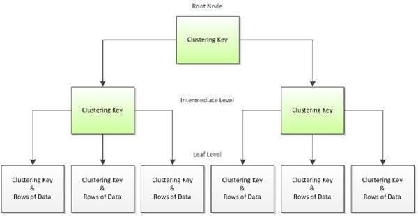
Figure 1: The b-tree structure of a clustered index

It can be helpful, when trying to remember which levels hold which information, to compare the B-tree to an actual tree. You can visualize the root node as the trunk of a tree, the intermediate levels as the branches of a tree, and the leaf level as the actual leaves on a tree.

The leaf level of the B-tree is always level 0, and the root level is always the highest level. Figure 1 shows only one intermediate level but the number of intermediate levels actually depends on the size of the table. A large index will often have more than one intermediate level, and a small index might not have an intermediate level at all.

Index pages in the root and intermediate levels contain the clustering key and a page pointer down into the next level of the B-tree. This pattern will repeat until the leaf node is reached. You’ll often hear the terms “leaf node” and “data page” used interchangeably, as the leaf node of a clustered index contains the data pages belonging to the table. In other words, the leaf level of a clustered index is where the actual data is stored, in an ordered fashion based on the clustering key.

Let’s look at the B-tree again. Figure 2 represents the clustered index structure for a fictional table with 1 million records and a clustering key on EmployeeID.

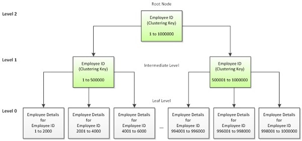
Figure 2: A b-tree index for a 1-million row table

The pages in Level 1 and Level 2, highlighted in green, are index pages. In Level 1, each page contains information for 500,000 records. As discussed, each of these pages stores not half a million rows, but rather half a million clustered index values, plus a pointer down into the associated page on the next level. For example, to retrieve the details for Employee 500, SQL Server would read three pages: the root page in Level 2, the intermediate page in Level 1, and the appropriate leaf level page in Level 0. The root page tells SQL Server which intermediate level page to read, and the intermediate page tells it which specific leaf level page to read.

In this manner, SQL Server uses a clustered index structure to retrieve the data requested by a query. For example, consider the following query against the Sales.SalesOrderHeader table in AdventureWorks, to return details of a specific order.

This table has a clustered index on the SalesOrderID column and SQL Server is able to use it to navigate down through the clustered index B-tree to get the information that is requested. If we were to visualize this operation, it would look something like this:

Root Node	SalesOrderID	PageID
	NULL	750
	59392	751
Intermediate level (Page 750)	SalesOrderID	PageID
	44150	814
	44197	815
	44244	816
	44290	817
	44333	818
Leaf level (Page 815)	SalesOrderID	OrderDate	SalesOrderNumber	AccountNumber	CustomerID
	44240	9/23/2005	SO44240	10-4030-013580	13580
	44241	9/23/2005	SO44241	10-4030-028155	28155
	44242	9/23/2005	SO44242	10-4030-028163	28163

In the root node, the first entry points to PageID 750, for any values with a SalesOrderID between NULL and 59391. The data we’re looking for, with a SalesOrderID of 44242, falls within that range, so we navigate down to page 750, in the intermediate level. Page 750 contains more granular data than the root node and indicates that the PageID 815 contains SalesOrderID values between 44197 and 44243. We navigate down to that page in the leaf level and, finally, upon loading PageID 815, we find all of our data for SalesOrderID 44242.

Characteristics of an effective clustered index

Based on this understanding of how a clustered index works, let’s now examine why and how this dictates the components of an effective clustered index key: narrow, unique, static, and ever-increasing.

Narrow

The width of an index refers to the number of bytes in the index key. The first important characteristic of the clustered index key is that it is as narrow as is practical. To illustrate why this is important, consider the following narrow_example table:

The table has been populated with 10 million rows and table contains two columns that are candidates for use as the clustering key:

• web_id – a fixed-length int data type, consuming 4 bytes of space
• web_key – a fixed-length uniqueidentifier data type, consuming 16 bytes.

So, which column will make a better clustered index key? Let’s take a look at the B-tree structure of each, shown in Figure 3.

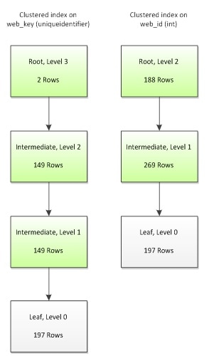
Figure 3: The b-tree levels for clustered indexes based on int and uniqueidenitifier key

The most obvious difference is that the uniqueidentifier key has an additional non-leaf level, giving 4 levels to its tree, as opposed to only 3 levels for the int key. The simple reason for this is that the uniqueidentifier consumes 300% more space than the int data type, and so when we create a clustered key on uniqueidentifier, fewer rows can be packed into each index page, and the clustered key requires an additional non-leaf level to store the keys.

Conversely, using a narrow int column for the key allows SQL Server to store more data per page, meaning that it has to traverse fewer levels to retrieve a data page, which minimizes the IO required to read the data. The potential benefit of this is large, especially for range scan queries, where more than one row is required to fulfill the query criteria. In general, the more data you can fit onto a page, the better your table can perform. This is why appropriate choice of data types is such an essential component of good database design.

However, our choice of clustering key can affect the performance of not only the clustered index, but also any non-clustered indexes that rely on the clustered index. As shown in Figure 4, a non-clustered index contains the clustered index key in every level of its b-tree structure, as a pointer back into the clustered index. This happens regardless of whether or not the clustering key was explicitly included in the nonclustered index structure, either as part of the index key or as an included column. In other words, whereas in the clustered index the leaf level contains the actual data rows, in a nonclustered index, the leaf level contains the clustered key, which SQL Server uses to find the rest of the data.

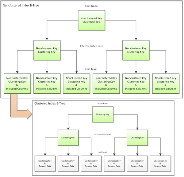
Figure 4: Non-clustered indexes also store the clustering key in order to look up data in the clustered index

So, let’s see how our choice of clustering key impacts the potential performance of our non-clustered indexes. We’ll keep the example pretty simple and create a non-clustered index on customer_id, which is an int data type.

Figure 5 shows the resulting B-tree structures of our nonclustered index, depending on whether we used the uniqueidentifier or the int column for our clustered index key.

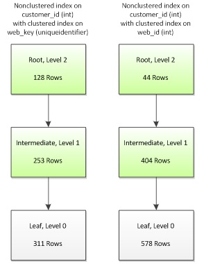
Figure 5

While we have the same number of levels in each version of the index, notice that the non-clustered index based on the int clustering key stores 86% more data in each leaf-level data page than its uniqueidentifier counterpart. Once again, the more rows you can fit on a page, the better the overall system performance: range-scan queries on the narrow int version will consume less IO and execute faster than equivalent queries on the wider, uniqueidentifier version.

In this example, I’ve kept the table and index structures simple in order to better illustrate the basic points. In a production environment, you’ll often encounter tables that are much, much wider. It’s possible that such tables will require a composite clustered index, where the clustering key is comprised of more than one column. That’s okay; the point isn’t to advise you to base all of your clustered keys on integer IDENTITY columns, but to demonstrate that a wide index key can have on a significant, detrimental impact on a database’s performance, compared to a narrow index key. Remember, narrowness refers more to the number of bytes consumed than the number of columns. For example, a composite clustered key on three int columns would still be narrower than a uniqueidentifier key (4 + 4 + 4 = 12 bytes for the former vs. 16 bytes for the latter).

Unique

Index uniqueness is another highly desirable attribute of a clustering key, and goes hand-in-hand with index narrowness. SQL Server does not require a clustered index to be unique, but yet it must have some means of uniquely identifying every row. That’s why, for non-unique clustered indexes, SQL Server adds to every duplicate instance of a clustering key value a 4-byte integer value called a uniqueifier. This uniqueifier is added everywhere the clustering key is stored. That means the uniqueifier is stored in every level of the B-tree, in both clustered and non-clustered indexes. As you can imagine, if there are many rows using the same clustering key value, this can become quite expensive.

What’s more, the uniqueifier is stored as a variable-length column. This is important because if a table does not already contain any other variable-length columns, each duplicate value is actually consuming 8-bytes of overhead: 4 bytes for the uniqueifier value and 4 bytes to manage variable-length columns on the row. The following example demonstrates this. We create a table with a non-unique clustered index, insert into it a single row, and then retrieve minimum and maximum record sizes (which currently refer to the same, single record) from the sys.dm_db_index_physical_stats DMV:

Although we only have a single column in the table, there is a minimum of 7 bytes of overhead per row, in SQL Server. While this overhead may increase with the addition of NULL or variable-length columns, it will never be less than 7 bytes per row. The other 4 bytes are used to store the int column, myID.

Now let’s insert a duplicate value into the table:

The duplicate value requires the addition of a uniqueifier, which consumes an extra 4 bytes. However, since a variable-length column, such as a varchar() column, does not already exist on the table, an additional 4 bytes are added by SQL Server to manage the variable-length properties of the uniqueifier. This brings the total uniqueifier overhead to 8 bytes per row.

So, returning to our original narrow_example table, let’s see what would happen if the clustering key was changed to customer_id, which is a non-unique int. Although the uniqueifier is not readily visible and cannot be queried, internally the leaf-level page might look something like this:

web_id	web_key	log_date	customer_id	uniqueifier
1	6870447C-A0EC-4B23-AE5F-9A92A00CE166	12/15/2010	1	NULL
2	5AB480CF-40CD-43FD-8C3D-5C625875E143	12/15/2010	1	1
3	95C312B9-83AF-4725-B53C-77615342D177	12/15/2010	1	2
4	88AA4497-9A20-4AB7-9704-1FDFAE200564	12/15/2010	2	NULL
5	E3EA3014-FC23-48B6-9205-EE6D06D37C5B	12/15/2010	2	1
6	9F6A8933-F6EC-416F-AACA-1C3FF172151C	12/15/2010	3	NULL
7	B16406A8-649B-4E7A-A234-C7B7D8FCE2D3	12/15/2010	4	NULL
8	443B627B-21CE-4466-AD15-1879C8749225	12/15/2010	4	1
9	2F3757DE-3799-4246-BA88-944C5DA3683E	12/15/2010	4	2
10	25D9F2AA-6610-48CD-9AC4-4F1E29FDED1C	12/15/2010	4	3

The uniqueifier is NULL for the first instance of each customer_id, and is then populated, in ascending order, for each subsequent row with the same customer_id value. The overhead for rows with a NULL uniqueifier value is, unsurprisingly, zero bytes. This is why min_record_size_in_bytes remained unchanged in the overhead table; the first insert had a uniqueifier value of NULL. This is also why it is impossible to estimate how much additional storage overhead will result from the addition of a uniqueifier, without first having a thorough understanding of the data being stored. For example, a non-unique clustered index on a datetime column may have very little overhead if data is inserted, say, once per minute. However, if that same table is receiving thousands of inserts per minute, then it is likely that many rows will share the same datetime value, and so the uniqueifier will have a much higher overhead.

If your requirements seem to dictate the use of a non-unique clustered key, my advice would be to look to see if there are a couple of relatively narrow columns that, together, can form a unique key. You’ll still see the increase in the row size for your clustering key in the index pages of both your clustered and nonclustered indexes, but you’ll at least save the cost of the uniqueifier in the data pages of the leaf level of your clustered index. Also, instead of storing an arbitrary uniqueifier value to the index key, which is meaningless in the context of your data, you would be adding meaningful and potentially useful information to all of your nonclustered indexes.

A good clustered index is also built upon static, or unchanging, columns. That is, you want to choose a clustering key that will never be updated. SQL Server must ensure that data exists in a logical order based upon the clustering key. Therefore, when the clustering key value is updated, the data may need to be moved elsewhere in the clustered index so that the clustering order is maintained. Consider a table with a clustered index on LastName, and two non-clustered indexes, where the last name of an employee must be updated.

Figure 6: The effect of updating a clustered key column

Not only is the clustered index updated and the actual data row moved – most likely to a new data page – but each non-clustered index is also updated. In this particular example, at least three pages will be updated. I say “at least” because there are many more variables involved, such as whether or not the data needs to be moved to a new page. Also, as discussed earlier, the upper levels of the B-tree contain the clustering key as pointers down into the leaf level. If one of those index pages happens to contain the clustering key value that is being updated, that page will also need to be updated. For now, though, let’s assume only three pages are affected by the UPDATE statement, and compare this to behavior we see for the same UPDATE, but with a clustering key on ID instead of LastName.

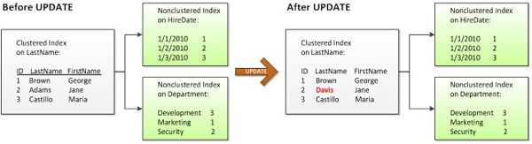
Figure 7: An UPDATE that does not affect the clustered index key

In Figure 7, only the data page in the clustered index is changed because the clustering key is not affected by the UPDATE statement. Since only one page is updated instead of three, clustering on ID requires less IO than clustering on LastName. Also, updating fewer pages means the UPDATE can complete in less time.

Of course, this is another simplification of the process. There are other considerations that can affect how many pages are updated, such as whether an update to a variable-length column causes the row to exceed the amount of available space. In such a case, the data would still need to be moved, although only the data page of the clustered index is affected; nonclustered indexes would remain untouched.

Nevertheless, updating the clustering key is clearly more expensive than updating a non-key column. Furthermore, the cost of updating a clustering key increases as the number of non-clustered indexes increases. Therefore, it is a best practice is to avoid clustering on columns that are frequently updated, especially in systems where UPDATE performance is critical.

Ever-Increasing

The last important attribute of a clustered index key is that it is ever-increasing. In addition to narrow, unique, and static, an integer identity column is an excellent example of an ever-increasing column. The identity property continuously increments by the value defined at creation, which is typically one. This allows SQL Server, as new rows are inserted, to keep writing to the same page until the page is full, then repeating with a newly allocated page.

There are two primary benefits to an ever-increasing column:

1. Speed of insert – SQL Server can much more efficiently write data if it knows the row will always be added to the most recently allocated, or last, page
2. Reduction in clustered index fragmentation – this fragmentation results from data modifications and can take the form of gaps in data pages, so wasting space, and a logical ordering of the data that no longer matches the physical ordering.

However, before we can discuss the effect of the choice of clustering key on insert performance and index fragmentation, we need to briefly review the types of fragmentation that can occur.

Internal and external index fragmentation

There are two types of index fragmentation, which can occur in both clustered and non-clustered indexes: extent (a.k.a. external) and page (a.k.a. internal) fragmentation. First, however, Figure 8 illustrates an un-fragmented index.

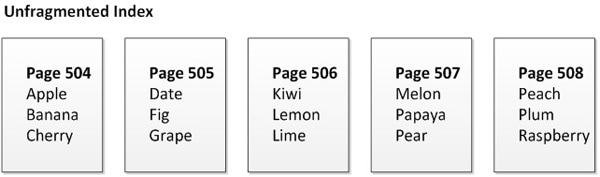
Figure 8: Data pages in an un-fragmented clustered index

In this simplified example, a page is full if it contains 3 rows, and in Figure 8 you can see that every page is full and the physical ordering of the pages is sequential. In extent fragmentation, also known as external fragmentation, the pages get out of physical order, as a result of data modifications. The pages highlighted in orange in Figure 9 are the pages that are externally fragmented. This type of fragmentation can result in random IO, which does not perform as well as sequential IO.

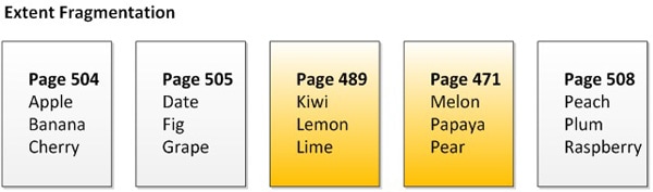
Figure 9: External fragmentation in a clustered index

Figure 10: Internal fragmentation in a clustered index

Figure 10 illustrates page fragmentation, also known as internal fragmentation, and refers to the fact that the there are gaps in the data pages, which reduces the amount of data that can be stored on each page, and so increase the overall amount of space needed to store the data. Again, the pages in orange indicate an internally fragmented page.

For example, comparing Figures 8 and 10, we can see that the un-fragmented index holds 15 data rows in 5 pages. By contrast, the index with internal fragmentation only holds 9 data rows in the same number of pages. This is not necessarily a big issue for singleton queries, where just a single record is needed to fulfill the request. However, when pages are not full and additional pages are required to store the data, range-scan queries will feel the effects, as more IO will be required to retrieve those additional pages.

Most indexes suffering from fragmentation will often have both extent and page fragmentation.

How non-sequential keys can increase fragmentation

Clustering on ever-increasing columns such as identity integers will result in an un-fragmented index, as illustrated in Figure 8. This results in sequential IO and maximizes the amount of data stored per page, resulting in the most efficient use of system resources. It also results in very fast write performance.

Use of a non-sequential key column can, however, result in a much higher overhead during insertion. First, SQL Server has to find the correct page to write to and pull it into memory. If the page is full, SQL Server will need to perform a page split to create more space. During a page split, a new page is allocated, and half the records are moved from the old page to the newly-allocated page. Each page has a pointer to the previous and next page in the index, so those pages will also need to be updated. Figure 11 illustrates the results of a page split.

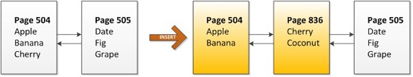
Figure 11: Internal and external fragmentation as a result of a page split

Initially, we have two un-fragmented pages, each holding 3 rows of data. However, a request to insert “coconut” into the table results in a page split, because Page 504, where the data naturally belongs, is full. SQL Server allocates a new page, Page 836, to store the new row. In the process, it also moves half the data from Page 504 to the new page in order to make room for new data in the future. Lastly, it updates the previous and next pointers in both pages 504 and 505. We’re left with Page 836 out of physical ordering, and both pages 504 and 836 contain free space. As you can see, not only would writes to this latter scenario be slower, but both internal and external fragmentation of the table would be much higher.

I once saw a table with 4 billion rows clustered on a non-sequential uniqueidentifier, also known as a GUID. The table had a fragmentation level of 99.999%. Defragging the table and changing the clustering key to an identity integer resulted in a space savings of over 200 GB. Extreme, yes, but it illustrates just how much impact an ever-increasing clustering key can have on table.

I am not suggesting that you only create clustered indexes on identity integer columns. Fragmentation, although generally undesirable, primarily impacts range-scan queries; singleton queries would not notice much impact. Even range-scan queries can benefit from routine defragmentation efforts. However, the ever-increasing attribute of a clustered key is something to consider, and is especially important in OLTP systems where INSERT speed is important.

Summary

In this article, I’ve discussed the most desirable attributes of a clustered index: narrow, unique, static, and ever-increasing. I’ve explained what each attribute is and why each is important. I’ve also presented the basics of B-tree structure for clustered and non-clustered indexes. The topic of “indexing strategy” is vast topic and we’ve only scratched the surface. Beyond what I presented in this article, there are also many application-specific considerations when choosing a clustering key, such as how data will be accessed and the ability to use the clustered index in range-scan queries. As such, I’d like to stress that the attributes discussed in this article are not concrete rules but rather time-proven guidelines. The best thing to do if you’re not sure if you’ve chosen the best clustering key is to test and compare the performance of different strategies.

Further Reading

• Brad’s Sure Guide to Indexes Brad McGehee’s “ground level” overview of indexes and how they work
• Defragmenting Indexes in SQL Server 2005 and 2008 Rob Sheldon on investigating, and fixing, index fragmentation using sys.dm_db_index_physical_stats.
• SQL Server Indexes: The Basics, by Kathi Kellenberger