There are many factors to consider when sizing and configuring the storage subsystem. It is very easy to hamstring an otherwise powerful system with poor storage choices. Important factors, discussed in this article, include:

• Disk seek time and rotational latency limitations
• Type of disk drive used:
  • Traditional magnetic drive – SATA, SCSI, SAS and so on
  • Solid State Drives (SSDs)
• Storage array type: Storage Area Network (SAN) vs. Direct Attached Storage (DAS)
• Redundant Array of Independent disk (RAID) configuration of your disks

Having reviewed each component of the disk subsystem, we’ll discuss how the size and nature of the workload will influence the way in which the subsystem is provisioned and configured.

Disk I/O

RAM capacity has increased unremittingly over the years and its cost has decreased enough to allow us to be lavish in its use for SQL Server, to help minimize disk I/O. Also, CPU speed has increased to the point where many systems have substantial spare capacity that can often be used to implement data compression and backup compression, again to help reduce I/O pressure. The common factor here is “helping to reduce disk I/O”. While disk capacity has improved greatly, disk speed has not, and this poses a great problem; most large, busy OLTP systems end up running into I/O bottlenecks.

The main factors limiting how quickly that data is returned from a single traditional magnetic disk is the overall disk latency, which breaks down as follows:

• Seek time – the time it takes the head to physically move across the disk to find the data. This will be a limiting factor in the number of I/O operations a single disk can perform per second (IOPS) that your system can support.
• Rotational latency – the time it takes for the disk to spin to read the data off of the disk. This is a limiting factor in the amount of data a single disk can read per second (usually measured in MB/s), in other words the I/O throughput of the that disk.

Typically, you will have multiple magnetic disks working together in some level of RAID to increase both performance and redundancy. Having more disk spindles (i.e. more physical disks) in a RAID array increases both throughput performance and IOPS performance.

However, a complicating factor here is the performance limitations of your RAID controllers, for direct attached storage, or Host Bus Adaptors (HBAs), for a storage area network. The throughput of such controllers, usually measured in gigabits per second, e.g. 3Gbps, will dictate the upper limit for how much data can be written or read from a disk per second. This can have a huge effect on your overall IOPS and disk throughput capacity for each logical drive that is presented to your host server in Windows.

The relative importance of each of these factors depends on the type of workload being supported; OLTP or DSS/DW. This in turn will determine how you provision the disk storage subsystem.

OLTP workloads are characterized by a high number of short transactions, where the data is tends to be rather volatile (modified frequently). There is usually much higher write activity in an OLTP workload than in a DSS workload. As such, most OLTP systems generate more input/output operations per second (IOPS) than an equivalent sized DSS system.

Furthermore, in most OLTP databases, the read/write activity is largely random, meaning that each transaction will likely require data from a different part of the disk. All of this means that in most OLTP applications, the hard disks will spend most of their time seeking data, and so the seek time of the disk is a crucial bottleneck for an OLTP workload. The seek time for any given disk is determined by how far away from the required data the disk heads are at the time of the read/write request.

A DSS or DW system is usually characterized by longer running queries than a similar size OLTP system. The data in a DSS system is usually more static, with much higher read activity than write activity. The disk activity with a DSS workload also tends to be more sequential and less random than with an OLTP workload. Therefore, for a DSS type of workload, sequential I/O throughput is usually more important than IOPS performance. Adding more disks will increase your sequential throughput until you run into the throughput limitations of your RAID controller or HBA. This is especially true when a DSS/DW system is being loaded with data, and when certain types of complex, long-running queries are executed.

Generally speaking, while OLTP systems are characterized by lots of fast disks, to maximize IOPS to overcome disk latency issues with high numbers of random reads and writes, DW/DSS systems require lots of I/O channels, in order to handle peak sequential throughput demands. An I/O channel is an individual RAID controller or an individual HBA; either of which gives you a dedicated, separate path to either a DAS array or a SAN. The more I/O channels you have, the better.

With all of this general advice in mind, let’s now consider each of the major hardware and architectural choices that must be made when provisioning the storage subsystem, including the type of disks used, the type of storage array, and the RAID configuration of the disks that make up the array.

Drive Types

Database servers have traditionally used magnetic hard drive storage. Seek times for traditional magnetic hard disks have not improved appreciably in recent years, and are unlikely to improve much in the future, since they are electro-mechanical in nature. Typical seek times for modern hard drives are in the 5-10ms range.

The rotational latency for magnetic hard disks is directly related to the rotation speed of the drive. The current upper limit for rotational speed is 15,000 rpm, and this limit has not changed in many years. Typical rotational latency times for 15,000 rpm drives are in the 3-4ms range.

This disk latency limitation lead to the proliferation of vast SAN (or DAS)-based storage arrays, allowing data to be striped across numerous magnetic disks, and leading to greatly enhanced IO throughput. However, in trying to fix the latency problem, SANs have become costly, complex and sometimes fault-prone. These SANs are generally shared by many databases, which adds even more complexity and often results in a disappointing performance, for the cost.

Newer solid state storage technology has the potential to displace traditional magnetic drives, and even SANs altogether, and allow for much simpler storage systems. The seek times for SSDs and other flash based storage is much, much lower than for traditional magnetic hard disks, since there are no electro-mechanical moving parts to wait on. With an SSD, there is no delay for an electro-mechanical drive head to move to the correct portion of the disk to start reading or writing data. With an SSD, there is no delay waiting for the spinning disk to rotate past the drive head to start reading or writing data, and the latency involved in reading data off of an SSD is much lower than it is for magnetic drives, especially for random reads and writes. SSD drives also have the additional advantage of lower electrical power usage, especially compared to large numbers of traditional magnetic hard drives.

Magnetic Disk Drives

Disks are categorized according to the type of interface they use. Two of the oldest types of interface, which you still occasionally see in older workstations, are Integrated Drive Electronics (IDE) or Parallel Advanced Technology Attachment (PATA) drives. Of course, it is not unusual for old, “retired” workstations, with PATA disk controllers, to be pressed into service as development or test database servers. However, I want to stress that you should not be using PATA drives for any serious database server use.

PATA and IDE drives are limited to two drives per controller, one of which is the Master and the other is the Slave. The individual drive needed to have a “Jumper Setting” to designate whether the drive was acting as a Master or a Slave drive. PATA 133 was limited to a transfer speed of 133MB/sec, although virtually no PATA drives could sustain that level of throughput.

Starting in 2003, Serial Advanced Technology Attachment (SATA) drives began replacing PATA drives in workstations and entry-level servers. They offer throughput capacities of 1.5, 3, or 6 Gbps (also commonly known as SATA 1.0, SATA 2.0, and SATA 3.0), along with hot-swap capability. Most magnetic SATA drives have a 7200rpm rotational speed, although a few can reach 10,000rpm. Magnetic SATA drives are often used for low-cost backup purposes in servers, since their performance and reliability typically does not match that of enterprise-level SAS drives.

Both traditional magnetic drives and newer SSDs can use the SATA interface. With an SSD, it is much more important to make sure you are using a 6Gbps SATA port, since the latest generation SSDs can completely saturate an older 3Gbps SATA port.

External SATA (eSATA) drives are also available. They require a special eSATA port, along with an eSATA interface to the drive itself. An eSATA external drive will have much better data transfer throughput than the more common external drives that use much slower USB 2.0 interface. The new USB 3.0 interface is actually faster than eSATA, but your throughput will be limited by the throughput limit of the external drive itself, not the interface.

Small Computer System Interface (SCSI) drives have been popular in server applications since the mid 1980’s. SCSI drives were much more expensive than PATA drives, but offered better performance and reliability. The original parallel SCSI interface is now being rapidly replaced by the newer Serial Attached SCSI (SAS) interface. Most enterprise-level database servers will use either parallel SCSI or SAS internal drives, depending on their age. Any new or recent-vintage database server will probably have SAS internal drives instead of SCSI internal drives.

Server class magnetic hard drives have rotation speeds ranging from 7200 rpm (for SATA) to either 10,000 rpm or 15,000 rpm (for SCSI and SAS). Higher rotation speeds reduce data access time by reducing the rotational latency. Drives with higher rotation speed are more expensive, and often have lower capacity sizes compared to slower rotation speed drives. Over the last several years disk buffer cache sizes have grown from 2MB all the way to 64MB. Larger disk buffers usually improve the performance of individual magnetic hard drives, but often are not as important when the drive is used by a RAID array or is part of a SAN, since the RAID controller or SAN will have its own, much larger cache that is used to cache data from multiple drives in the array.

Solid State Drives

Solid State Drives (SSD), or Enterprise Flash Disks (EFD), are different from traditional magnetic drives in that they have no spinning platter, drive actuator, or any other moving parts. Instead, they use flash memory, along with a storage processor, controller and some cache memory, to store information.

The lack of moving parts eliminates the rotational latency and seek-time delay that is inherent with a traditional magnetic hard drive. Depending on the type of flash memory, and the technology and implementation of the controller, SSDs can offer dramatically better performance compared to even the fastest enterprise-class magnetic hard drives. This performance does come at a much higher cost per gigabyte, and it is still somewhat unusual for database servers, direct attached storage or SANs, to exclusively use SSD storage, but this will change as SSD costs continue to decrease.

SSDs perform particularly well for random access reads and writes, and for sequential access reads. Some earlier SSDs do not perform as well for sequential access writes, and they also have had issues where write performance declines over time, particularly as the drive fills up. Newer SSD drives, with better controllers and improved firmware, have mitigated these earlier problems.

There are two main types of flash memory currently used in SSDs: Single Level Cell (SLC) and Multi Level Cell (MLC). Enterprise level SSDs almost always use SLC flash memory since MLC flash memory does not perform as well and is not as durable as the more-expensive SLC flash memory.

Fusion-IO Drives

Fusion-IO is a company that makes several interesting “SSD-like” products that are getting a lot of visibility in the SQL Server community. The term “SSD-like” refers to Fusion-IO cards that use flash memory, just like SSDs do, but are connected to your server through a PCI-E slot, instead of a SAS or SATA controller.

The Fusion-IO products are relatively expensive, but offer extremely high performance. Their three current server-related products are the ioDrive, ioDrive Duo and the new ioDrive Octal. All three of these products are PCI-E cards, with anywhere from 80GB to 5.12TB of SLC or MLC flash on a single card. Using a PCI-E expansion slot gives one of these cards much more bandwidth than a traditional SATA or SAS connection. The typical way to use Fusion-IO cards is to have at least two of the cards, and then to use software RAID in Windows to get additional redundancy. This way, you avoid having a pretty important single point of failure, in the card itself and the PCI-E slot it was using (but incur the accompanying increase in hardware expenditure).

Fusion-IO drives offer excellent read and write performance, albeit at a relatively high hardware cost. As long as you have enough space, it is possible and feasible to locate all of your database components on Fusion-IO drives, and get extremely good I/O performance, without the need for a SAN. One big advantage of using Fusion-IO, instead of a traditional SAN, is the reduced electrical power usage and reduced cooling requirements, which are big issues in many data centers.

Since Fusion-IO drives are housed in internal PCI-E slots in a database server, you cannot use them with traditional Windows Fail-Over Clustering (which requires shared external storage for the cluster), but you can use them with database mirroring or the upcoming AlwaysOn technology in SQL Server Denali, which allows you to create a Windows Cluster with no shared storage.

SSDs and SQL Server

I’m often asked which components of a SQL Server database should be moved to SSD storage, as they become more affordable. Unfortunately, the answer is that it depends on your workload, and on where (if anywhere) you are experiencing I/O bottlenecks in your system (data files, TempDB files, or transaction log file).

Depending on your database size, and your budget, it may make sense to move the entire database to solid state storage, especially with a heavy OLTP workload. For example, if your database(s) are relatively small, and your budget is relatively large, it may be feasible to have your data files, your log files, and your TempDB files all running on SSD storage.

If your database is very large, and your hardware budget is relatively small, you may have to be more selective about which components can be moved to SSD storage. For example, it may make sense to move your TempDB files to SSD storage if your TempDB is experiencing I/O bottlenecks. Another possibility would be to move some of your most heavily accessed tables and indexes to a new data file, in a separate file group, that would be located on your SSD storage.

Internal Storage

All blade and rack-mounted database servers have some internal drive bays. Blade servers usually have two to four internal drive bays, while rack servers have higher numbers of drive bays, depending on their vertical size. For example, a 2U server will have more internal drive bays than an equivalent 1U server (from the same manufacturer and model line). For standalone SQL Server instances, it is common to use at least two 15K drives in RAID 1 for the operating system and SQL Server binaries. This provides a very basic level of redundancy for the operating system and the SQL Server binaries, meaning that the loss of a single internal drive will not bring down the entire database server.

Modern servers often use 2.5″ drives, in place of the 3.5″ drives that were common a few years ago. This allows more physical drives to fit in the same size chassis, and it reduces the electrical and cooling requirements. The latest 2.5″ drives also tend to out-perform older 3.5″ drives. Despite these improvements, however, for all but very lightest database workloads, you simply won’t have enough internal drive bays to completely support your I/O requirements.

Ignoring this reality is a very common mistake that I see made by many DBAs and companies. They buy a new, high performance database server with fast multi-core processors and lots of RAM and then try to run an OLTP workload on six internal drives. This is like a body-builder who only works his upper body, but completely neglects his legs, ending up completely out of balance, and ultimately not very strong. Most production SQL Server workloads will require much more I/O capacity than is available from the available internal drives. In order to provide sufficient storage capacity, and acceptable IO performance, additional redundant storage is required, and there are several ways to provide it.

Attached Storage

The two most common form of storage array used for SQL Server installations are Direct Attached Storage (DAS) and the Storage Area Network (SAN).

Direct Attached Storage (DAS)

One option is to use Direct Attached Storage (DAS), which is also sometimes called locally attached storage. DAS drives are directly attached to a server with an eSATA, SAS, or SCSI cable. Typically, you have an external enclosure, containing anywhere from 8 to 24 drives, attached to a RAID controller in single database server. Since DAS enclosures are relatively affordable compared to a Storage Area Network, it is becoming more common to use DAS storage, with multiple enclosures and multiple RAID controllers, to achieve very high throughput numbers for DW and Reporting workloads.

However, with relative simplicity and low cost, you do give up some flexibility. It is relatively hard to add capacity and change RAID levels when using DAS, compared to SAN.

The diagram in Figure 1 shows a somewhat simplified view of a server that is using Direct Attached Storage (DAS).

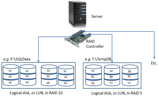
Figure 1: DAS Storage

You have a server with one or more PCI-e RAID controller cards that are connected (via a SAS or SCSI cable) to one or more external storage enclosures that usually have between 14 and 24 SAS or SCSI hard drives. The RAID controller(s) in the server are used to create and manage any RAID arrays that you decide to create and present to Windows as logical drives (that show up with a drive letter in Windows Explorer). This lets you build a storage subsystem with very good performance, relatively inexpensively.

Storage Area Network (SAN)

If you have a bigger budget, the next level of storage is a Storage Area Network (SAN). A SAN is a dedicated network that has multiple hard drives (anywhere from dozens to hundreds of drives) with multiple storage processors, caches, and other redundant components.

With the additional expense of the SAN, you do get a lot more flexibility. Multiple database servers can share a single, large SAN (as long as you don’t exceed the overall capacity of the SAN), and most SANs offer features that are not available with DAS, such as SAN snapshots. There are two main types of SANs available today: Fiber Channel and iSCSI.

A Fiber Channel SAN has multiple components, including large numbers of magnetic hard drives or solid state drives, a storage controller, and an enclosure to hold the drives and controller. Some SAN vendors are starting to use what they call tiered storage, where they have some SSDs, some fast 15,000rpm Fiber Channel drives, and some slower 7200rpm SATA drives in a single SAN. This allows you to prioritize your storage, based on the required performance. For example, you could have your SQL Server transaction log files on SSD storage, your SQL Server data files on Fiber Channel storage, and your SQL Server backup files on slower SATA storage.

Multiple fiber channel switches, and host bus adapters (HBAs) connect the whole infrastructure together in what is referred to as a fabric. Each component in the fabric has a bandwidth capacity, which is typically 1, 2, 4 or 8 Gbits/sec. When evaluating a SAN, be aware of the entire SAN path (HBA, switches, caches, storage processor, disks, and so on), since a lower bandwidth component (such as a switch) mixed in with higher capacity components will restrict the effective bandwidth that is available to the entire fabric.

An iSCSI SAN is similar to a Fiber Channel SAN except that it uses a TCP/IP network, connected with standard Ethernet network cabling and components, instead of fiber optics. The supported Ethernet wire speeds that can be used for iSCSI include 100Mb, 1Gb, and 10Gb/sec. Since iSCSI SANs can use standard Ethernet components, they are usually much less expensive than Fiber Channel SANs. Early iSCSI SANs did not perform as well as contemporary Fiber Channel SANs, but that gap has closed in recent years.

One good option for an iSCSI SAN is to use a TCP Offload Engine, also known as a “TOE Card” instead of a full iSCSI host bus adapter (HBA). A TOE offloads the TCP/IP operations for that card from the main CPU, which can improve overall performance (for a slightly higher hardware cost).

Regardless of which type of SAN you evaluate or use, it is very important to consider multi-path IO (MPIO) issues. Basically, this means designing and implementing a SAN to eliminate any single point of failure. For example, you would start with at least two HBAs (preferably with multiple channels), connected to multiple switches, which are connected to multiple ports on the SAN enclosure. This gives you redundancy and potentially better performance (at a greater cost).

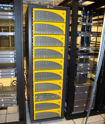
If you want to see what a “real life” SAN looks like, Figure 2 shows a 3PAR S400 SAN with (216) 146GB 10,000 rpm Fiber Channel drives and (24) 500GB 7,200 rpm SATA drives in a single, 42U rack enclosure. This SAN cost roughly $500,000 when it was purchased in 2006.

Figure 2: NewsGator’s 3PAR S400 SAN

RAID Configurations

Redundant array of independent disks (RAID) is a technology that allows use of multiple hard drives, combined in various ways, to improve redundancy, availability and performance, depending on the RAID level used. When a RAID array is presented to a host in Windows, it is called a logical drive.

Using RAID, the data is distributed across multiple disks in order to:

• Overcome the I/O bottleneck of a single disk, as described previously
• Get protection from data loss through the redundant storage of data on multiple disks
• Avoid any one hard drive being a single point of failure
• Manage multiple drives more effectively

Regardless of whether you are using traditional magnetic hard drive storage or newer solid state storage technology, most database servers will employ RAID technology. RAID improves redundancy, improves performance, and makes it possible to have larger logical drives. RAID is used for both OLTP and DW workloads. Having more spindles in a RAID array helps both IOPS and throughput, although ultimately throughput can be limited by a RAID controller or HBA.

Please note that while RAID does provide redundancy in your data storage, it is not a substitute for an effective backup strategy or a high availability/disaster recovery (HA/DR) strategy. Regardless of what level of RAID you use in your storage subsystem, you still need to run SQL Server full and log backups as necessary to meet your recovery point objectives (RPO) and recovery time objectives (RTO).

There are a number of commercially-available RAID configurations, which we’ll review over the coming sections, and each has associated costs and benefits. When considering which level of RAID to use for different SQL Server components, you have to carefully consider your workload characteristics, keeping in mind your hardware budget. If cost is no object, I am going to want RAID 10 for everything, i.e. data files, log file, and TempDB. If my data is relatively static, I may be able to use RAID 5 for my data files.

During the discussion, I will assume that you have a basic knowledge of how RAID works, and what the basic concepts of striping, mirroring, and parity mean.

RAID 0 (disk striping with no parity)

RAID 0 simply stripes data across multiple physical disks. This allows reads and writes to happen simultaneously, across all of the striped disks, so offering improved read and write performance, compared to a single disk. However, it actually provides no redundancy whatsoever. If any disk in a RAID 0 array fails, the array is off-line and all of the data in the array is lost. This is actually more likely to happen than if you only have a single disk, since the probability of failure for any single disk goes up as you add more disks. There is no disk space loss for storing parity data (since there is no parity data with RAID 0), but I don’t recommend that you use RAID 0 for database use, unless you enjoy updating your resume. RAID 0 is often used by serious computer gaming enthusiasts in order to reduce the time it takes to load portions of their favorite games. They do not keep any important data on their “gaming rigs”, so they are not that concerned about losing one of their drives.

RAID 1 (disk mirroring or duplexing)

You need at least two physical disks for RAID 1. Your data is mirrored between the two disks, i.e. the data on one disk is an exact mirror of that on the other disk. This provides redundancy, since you can lose one side of the mirror without the array going off-line and without any data loss, but at the cost of losing 50% of your space to the mirroring overhead. RAID 1 can improve read performance, but can hurt write performance in some cases, since the data has to be written twice.

On a database server, it is very common to install the Windows Server operating system on two (at least) of the internal drives, configured in a RAID 1 array, and using an embedded internal RAID controller on the motherboard. In the case of a non-clustered database server, it is also common to install the SQL Server binaries on the same two drive RAID 1 array as the operating system. This provides basic redundancy for both the operating system and the SQL Server binaries. If one of the drives in the RAID 1 array fails, you will not have any data loss or down-time. You will need to replace the failed drive and rebuild the mirror, but this is a pretty painless operation, especially compared to reinstalling the operating system and SQL Server!

RAID 5 (striping with parity)

RAID 5 is probably the most commonly-used RAID level, for both general file server systems and for SQL Server. RAID 5 requires at least three physical disks. The data, and calculated parity information, is striped across the physical disks by the RAID controller. This provides redundancy because if one of the disks goes down, then the missing data from that disk can be reconstructed from the parity information on the other disks. Also, rather than losing 50% of your storage, in order to achieve redundancy, as for disk mirroring, you only lose 1/N of your disk space (where N equals the number of disks in the RAID 5 array) for storing the parity information. For example, if you had six disks in a RAID 5 array, you would lose 1/6th of your space for the parity information.

However, you will notice a very significant decrease in performance while you are missing a disk in a RAID 5 array, since the RAID controller has to work pretty hard to reconstruct the missing data. Furthermore, if you lose a second drive in your RAID 5 array, the array will go offline, and all of the data will be lost. As such, if you lose one drive, you need to make sure to replace the failed drive as soon as possible. RAID 6 stores more parity information than RAID 5, at the cost of an additional disk devoted to parity information, so you can survive losing a second disk in a RAID 6 array.

Finally, there is a write performance penalty with RAID 5, since there is overhead to write the data, and then to calculate and write the parity information. As such, RAID 5 is usually not a good choice for transaction log drives, where we need very high write performance. I would also not want to use RAID 5 for data files where I am changing more than 10% of the data each day. One good candidate for RAID 5 is your SQL Server backup files. You can still get pretty good backup performance with RAID 5 volumes, especially if you use backup compression.

RAID 10 and RAID 0+1

When you need the best possible write performance, you should consider either RAID 0+1 or, preferably, RAID 10. These two RAID levels both involve mirroring (so there is a 50% mirroring overhead) and striping but differ in the details in how it is done in each case.

In RAID 10 (striped set of mirrors), the data is first mirrored and then striped. In this configuration, it is possible to survive the loss of multiple drives in the array (one from each side of the mirror), while still leaving the system operational. Since RAID 10 is more fault tolerant than RAID 0+1, it is preferred for database usage.

In RAID 0+1 (mirrored pair of stripes) the data is first striped, and then mirrored. This configuration cannot handle the loss of more than one drive in each side of the array.

RAID 10 and RAID 0+1 offer the highest read/write performance, but incur a roughly 100% storage cost penalty, which is why they are sometimes called “rich man’s RAID”. These RAID levels are most often used for OLTP workloads, for both data files and transaction log files. As a SQL Server database professional, you should always try to use RAID 10 if you have the hardware and budget to support it. On the other hand, if your data is less volatile, you may be able to get perfectly acceptable performance using RAID 5 for your data files. By “less volatile”, I mean if less than 10% of your data changes per day, then you may still get acceptable performance from RAID 5 for your data files(s).

RAID Controllers

There are two common types of hardware RAID controllers used in database servers. The first is an integrated hardware RAID controller, embedded on the server motherboard. This type of RAID controller is usually used to control internal drives in the server. The second is a hardware RAID controller on a PCI-E expansion card that slots into one of the available, and compatible, PCI-E expansion slots in your database server. This is most often used to control one or more direct attached storage enclosures, which are full of SAS, SATA or SCSI hard drives.

It is also possible to use the software RAID capabilities built into the Windows Server operating system, but I don’t recommend this for production database use with traditional magnetic drives, since it places extra overhead on the operating system, is less flexible, has no dedicated cache, and increases the load on the processors and memory in a server. For both internal drives and direct attached storage, dedicated hardware RAID controllers are much preferable to software RAID. One exception to this guidance is if you are going to use multiple Fusion-IO drives in a single database server, in which case it is acceptable, and common to use software RAID.

Hardware-based RAID uses a dedicated RAID controller to manage the physical disks that are part of any RAID arrays that have been created. A server-class hardware RAID controller will have a dedicated, specialized processor that is used to calculate parity information; this will perform much better than using one of your CPUs for that purpose. Besides, your CPUs have more important work to do, so it is much better to offload that work to a dedicated RAID controller.

A server-class hardware RAID controller will also have a dedicated memory cache, usually around 512MB in size. The cache in a RAID controller can be used for either reads or writes, or split between the two purposes. This cache stores data temporarily, so that whatever wrote that data to the cache can return to another task without having to wait to write the actual physical disk(s).

Especially for database server use, it is extremely important that this cache is backed up by a battery, in case the server ever crashes or loses power before the contents of the RAID controller cache are actually written to disk. Most RAID controllers allow you to control how the cache is configured, in terms of whether it is used for reads or writes or a combination of the two. Whenever possible, you should disable the read cache (or reduce it to a much smaller size) for OLTP workloads, as they will make little or no use of it. By reducing the read cache you can devote more space, or often the entire cache, to write activity, which will greatly improve write performance. You can also usually control whether the cache is acting as a write-back cache or a write-through cache. In a write-through cache, every write to the cache causes a synchronous write to the backing store, which is safer, but reduces the write performance of the cache. A write-back cache improves write performance, because a write to the high-speed cache is faster than to the actual disk(s). As enough of the data in the write-back cache becomes “dirty”, it will eventually have to actually be written to the disk subsystem. The fact that data that has been marked as committed by database is still just in the write-back cache is why it is so critical to have a battery backing the cache.

For both performance and redundancy reasons, you should always try to use multiple HBAs or RAID controllers whenever possible. While most direct attached storage enclosures will allow you to “daisy-chain” multiple enclosures on a single RAID controller, I would avoid this configuration, if possible, since the RAID controller will be a single point of failure, and possibly a performance bottleneck as you approach he throughput limit of the controller. Instead, I would want to have one RAID controller per DAS array (subject to the number of PCI-E slots you have available in your server). This gives you both better redundancy and better performance. Having multiple RAID controllers allows you to take advantage of the dedicated cache in each RAID controller, and helps ensure that you are not limited by the throughput capacity of the single RAID controller or the expansion slot that it is using.

Provisioning and Configuring the Storage Subsystem

Having discussed each of the basic components of the storage system, it’s time to review the factors that will determine the choices you make when provisioning and configuring the storage subsystem

The number, size, speed and configuration of the disks that comprise your storage array will be heavily dependent on size and nature of the workload. Every time that data required by an application or query is not found in the buffer cache, it will need to be read from the data files on disk, causing read I/O. Every time data is modified by an application, the transaction details are written to the transaction log file, and then the data itself is written to the data files on disk, causing write I/O in each case.

In addition to the general read and write I/O generated by applications that access SQL Server, additional I/O load will be created by other system and maintenance activities such as:

• Transaction log backups – create both read and write I/O pressure. The active portion of the transaction log file is read, and then the transaction log backup file must be written.
• Index maintenance, including index reorganizations and index rebuilds – create read I/O pressure as the index is read off of the I/O subsystem, which then causes memory pressure as the index data goes into the SQL Server Buffer Pool. There is CPU pressure as the index is reorganized or rebuilt and then write I/O pressure as the index is written back out to the I/O subsystem.
• Full text catalog and indexes for Full Text Search – the work of “crawling” the base table(s) to create and maintain these structures and then writing the changes to the Full Text index(s) creates both read and write I/O pressure.
• Database checkpoint operations – the write activity to the data files occurs during database checkpoint operations. The frequency of checkpoints is influenced by the recovery interval setting and the amount of RAM installed in the system.
• Use of High Availability/Disaster Recovery (HA/DR) – features like Log Shipping or Database Mirroring will cause additional read activity against your transaction log, since the transaction log must be read before the activity can be sent to the Log Shipping destination(s) or to the database mirror. Using Transactional Replication will also cause more read activity against your transaction log on your Publisher database.

The number of disks that make up your storage array, their specifications in terms of size, speed and so on, and the physical configuration of these drives, in the storage array, will be determined by the size of the I/O load that your system needs to support, both in terms of IOPS and I/O throughput, as well as in the nature of that load, in terms of the read I/O and write I/O activity that it generates.

A workload that is primarily “OLTP” in nature will generate a high number of I/O operations (IOPS) and a high percentage of write activity; it is not that unusual to actually have more writes than reads in a heavy OLTP system. This will cause heavy write (and read) IO pressure on the logical drive(s) that house your data files and, particularly, heavy write pressure on the logical drive where your transaction log is located, since every write must go to the transaction log first. The drives that house these files must be sized, spec’d and configured appropriately, to handle this pressure.

Furthermore, almost all of the other factors that cause additional I/O pressure, listed previously, are almost all more prominent for OLTP systems. High write activity, caused by frequent data modifications, leads to more regular transaction log backups, index maintenance, more frequent database checkpoints, and so on.

Backup and data compression
Using Data and Backup Compression can reduce the I/O cost and duration of SQL Server backups at the cost of some additional CPU pressure – see Chapter 1 in my book, SQL Server Hardware, for further discussion.

A DSS or DW system usually has longer running queries than a similar size OLTP system. The data in a DSS system is usually more static, with much higher read activity than write activity. The less-volatile data means less frequent data and transaction log backups – you might even be able to use read-only file groups to avoid having to regularly backup some file groups – less frequent index maintenance and so on, all of which contributes to a lower I/O load in terms of IOPS, though not necessarily I/O throughput, since the complex, long-running aggregate queries that characterize a DW/DSS workload will often read a lot of data, and the data load operations will write a lot of data. All of this means that for a DSS/DW type of workload, I/O throughput is usually more important than IOPS performance.

Finding the read/write ratio

One way of determining the size and nature of your workload is to retrieve the read/write ratio for your database files. The higher the proportion of writes, the more “OLTP-like” is your workload.

The DMV query shown in Listing 1 can be run on an existing system to help characterize the I/O workload for the current database. This query will show the read/write percentage, by file, for the current database, both in the number of reads and writes and in the number of bytes read and written.

Listing 1: Finding the read/write ratio, by file, for a given database

Three more DMV queries, shown in Listing 2, can help characterize the workload on an existing system from a read/write perspective, for cached stored procedures. These queries can help give you a better idea of the total read and write I/O activity, the execution count, along with the cached time for those stored procedures.

Listing 2: The read/write ratio for cached stored procedures

As discussed, a workload with a high percentage of writes will place more stress on the drive array where the transaction log files for your user databases is located, since all data modifications are written to the transaction log. The volatile the data, the more write I/O pressure you will see on your transaction log file. A workload with a high percentage of writes will also put more I/O pressure on your SQL Server data file(s). It is common practice with large volatile databases to have multiple data files spread across multiple logical drives to get both higher throughput and better IOPS performance. Unfortunately, you cannot increase I/O performance for your transaction log by adding additional files, since the log file is written to sequentially.

The relative read/write ratio will also affect how you configure the cache in your RAID controllers. For OLTP workloads, write cache is much more important than read cache, while read cache is more useful for DSS/DW workloads. In fact, it is a common best practice to devote the entire RAID controller cache to writes for OLTP workloads.

How many Disks?

One common mistake that you should avoid in selecting storage components is to only consider space requirements when looking at sizing and capacity requirements. For example, if you had a size requirement of 1TB for a drive array that was meant to hold a SQL Server data file, you could satisfy the size requirement by using three 500GB drives in a RAID 5 configuration. Unfortunately, for the reasons discussed, relating to disk latency, the performance of that array would be quite low. A better solution from a performance perspective would be to use either 8x146GB drives in RAID 5, or 15x73GB drives in RAID 5 to satisfy the space requirement with many more spindles. You should always try to maximize your spindle count instead of just using the minimum number of drives to meet a size requirement with the level of RAID you are going to use. So after all of this discussion, how many disks do you actually need to achieve acceptable performance?

Here is one formula for estimating the number of disks required for a given workload and RAID level that Australian SQL Server MVP Rod Colledge has written about:

It is important to consider both IOPS, to calculate the number of disks needed, and the I/O type, to ensure the I/O bus is capable of handling the peak I/O sequential throughput.

Configuration: SAN vs. DAS, RAID levels

For OLTP systems, the seek time and rotational latency limitations for a single disk, discussed at the start of this article, have led to the proliferation of large SAN-based storage arrays, allowing data to be segmented across numerous disks, in various RAID configurations. Many larger SANs have a huge number of drive spindles and so this architecture is able to support a very high random I/O rate (IOPS). Use of a SAN for the I/O subsystem, in OLTP workloads, makes it relatively easy (but expensive) to support dozens to hundreds of disk spindles for a single database server.

The general guideline is that you will get roughly 100 IOPS from a single 10,000rpm magnetic drive and about 150 IOPS from a single 15,000rpm drive. For example, if you had a SAN with two hundred 15,000rpm drives, that would give the entire SAN a raw IOPS capacity of 30,000 IOPS. If the HBAs in your database server were older 4Gbps models, your sequential throughput would still be limited to roughly 400MB/second for each HBA channel.

If you don’t have the budget or in-house expertise for a large SAN, it is still possible to get very good IOPS performance with other storage techniques such as using multiple direct attached storage (DAS) enclosures with multiple RAID controllers along with multiple SQL Server file groups and data files which allows you to spread the I/O workload among multiple logical drives that each represent a dedicated DAS enclosure. You can also use Solid State Drives (SSD) or Fusion-IO cards to get extremely high IOPS performance without using a SAN, assuming you have the hardware budget available to do that.

When you are using non-SAN storage (such as DAS enclosures) it is very important to explicitly segregate your disk activity by logical drive. This means doing things like having one or more dedicated logical drives for SQL Server data files, a dedicated logical drive for the log file (for each user database, if possible), a dedicated logical drive for your TempDB data and log files, and one or more dedicated logical drives for your SQL Server backup files. Of course your choices and flexibility are ultimately limited by the number of drives that you have available, which is limited by the number of DAS enclosures you have and the number of drives in each enclosure.

However, for DW/DSS systems, a SAN storage array may not be the best choice. Here, I/O throughput is the most important factor, and the throughput of a SAN array can be limited to the throughput capacity of a switch or individual host bus adapter (HBA). As such, it is becoming more common for DW/DSS systems to use multiple DAS devices, each on a dedicated RAID controller to get high levels of throughput at a relatively low cost.

If you have the available budget, I would prefer to use RAID 10 for all of your various SQL Server files, including data files, log files, TempDB, and backup files. If you do have budget constraints, I would consider using RAID 5 for your database backup files, and using RAID 5 for your data files (if they are relatively static). Depending on your workload characteristics and how you use TempDB, you might be able to use RAID 5 for TempDB files. I would fight as hard as possible to avoid using RAID 5 for transaction log files, since RAID 5 does not perform nearly as well for writes.

Summary

Having an appropriate storage subsystem is critical for SQL Server performance. Most high volume SQL Server workloads ultimately run into I/O bottlenecks that can be very expensive to alleviate. Selecting, sizing and configuring your storage subsystem properly will reduce the chances that you will suffer from I/O performance problems.

In addition, using powerful multi-core processors and large quantities of RAM is a relatively cheap extra protection from expensive I/O bottlenecks. Having more RAM reduces read I/O pressure, since more data can fit into the SQL Server buffer cache, and it can also reduce write I/O pressure by reducing the frequency of checkpoints. Using modern, multi-core processors can give you the excess processor capacity that can allow you to use various compression features, such as data compression and backup compression, which can also reduce I/O pressure in exchange for additional CPU utilization.

Ultimately, however, the only way to know that your chosen hardware, including the processor, disk subsystem and so on, is capable of handling the expected workload is to perform benchmark tests.

This is taken from Chapter 2 of Glen Berry’s book ‘SQL Server Hardware’, which is available from Amazon