SQL Server Integration Services (SSIS) can be a handy tool for developing and implementing extract, transform, and load (ETL) solutions, but getting started with SSIS can seem a daunting task, especially if you’re new to SSIS and ETL concepts. In such cases, it can help to see examples of how to build SSIS packages that carry out basic ETL operations.

This article provides such an example. In addition to introducing you to SSIS concepts and components, the article demonstrates how to use those components to develop an SSIS solution that extracts data from a file, transforms the data, and loads it into SQL Server.

To work through the examples in this article, you must be running Visual Studio with SQL Server Data Tools (SSDT) installed, a topic that has caused no end of confusion (and controversy) among SQL Server developers, some of whom still mourn the demise of Business Intelligence Development Studio (BIDS). If you’re running SQL Server 2008 or 2008 R2 and have access to BIDS, you’ll find that many of the concepts discussed here still apply, but the article is concerned primarily with SSIS development as it is implemented in SSDT, Microsoft’s current go-to tool for SSIS development.

For those of you not sure how to install SSDT in Visual Studio, you can refer to the following MSDN articles to help you get started:

• Install SQL Server Data Tools
• SQL Server Data Tools in Visual Studio 2015.

Once you have SSDT and Visual Studio set up the way you want them, you can start working through the examples in this article. I developed the examples based on the AdventureWorks2014 database, running on a local instance of SQL Server 2014. To try out the example for yourself, you must have access to a SQL Server instance, preferably with the AdventureWorks2014 database installed. You can probably get away with an earlier version of the database, but I haven’t tested that for myself.

Getting Started

There are two preliminary steps you must take in order to try out the examples in this article. The first is to run a bcp command similar to the following to export sample data to a text file:

The command retrieves data from the vEmployee view and saves it to the EmployeeData.txt file, which will be used as the source data for our SSIS package. Notice the -t argument included in the command, followed by the comma. This indicates that a comma will be used to delimit that values. Before you run the command, be sure to substitute the correct file path and SQL Server instance name, as appropriate for your environment.

The next step you must take is to create two tables (in the AdventureWorks2014 database, just to keep things simple). I used SQL Server Management Studio (SSMS) to create the tables, but you can instead use SSDT if you’re already familiar with the toolkit. In either environment, you should use the following CREATE TABLE statements to add the tables to the database:

The tables are nearly identical. The EmpSales table will store data about sales representatives, and the EmpNonSales table will store data about all other employees. The major difference between the two tables is that the EmpSales table includes the SalesGroup column, but the EmpNonSales table does not.

The tables will serve as the target for our ETL operation. We will retrieve the data from the EmployeeData.txt file, transform the data, and load it into the tables, taking a couple other steps along the way.

Creating an SSIS project

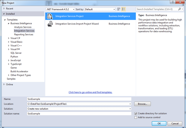
The first step in building our SSIS solution is to create an SSIS project in SSDT, based on the Integration Services Project template. To create the project, open Visual Studio, click the File menu, point to N ew, and then click Project.

In the New Project dialog box, navigate to the Integration Services node (one of the Business Intelligence templates), and select Integration Service s Project. In the bottom section of the dialog box, provide a project and solution name and specify a location for the project, as shown in the following figure.

When you click OK, Visual Studio generates the initial project files, which include a package file, named Package.dtsx. If you have the Solution Explorer pane open (shown in the following figure), you can see the project structure that has been created.

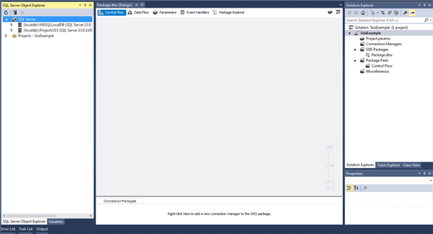
The package file provides a container for adding and configuring the components that carry out the ETL operation. We can rename the package file or add more package files, or simply stick with what we have, which is what we’ll do for this article.

The initial package file opens by default when we create our solution. SSDT provides a design surface (main window in the figure above) for working with the components within the file. We’ll be discussing the design surface in more detail as we work through our examples.

The figure above also shows the SQL Server Object Explorer pane for accessing SQL Server instances, much like you can in the Object Explorer pane in SQL Server Management Studio. You might or might not have this pane open on your system, which does not matter for what we’ll be doing here. What you will need, however, is the SSIS Toolbox pane, which is different from the default Visual Studio Toolbox pane.

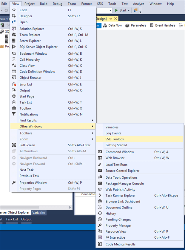
The SSIS Toolbox pane provides the components we need for defining our ETL operation, much like the Toolbox pane in BIDS. However, finding the option to open the SSIS Toolbox pane can be a bit tricky. To do so, click the View menu, point to Other Windows, and then click SSIS Toolbox, as shown in the following figure.

When I first tried this in Visual Studio 2015, the SSIS Toolbox option did not appear. I assumed that I was looking in the wrong place. I was not. I had to re-launch Visual Studio several times before the option appeared. When I tried to replicate this behavior, the results seemed inconsistent. I do not know whether this was a quirk with my system, with SSDT, or with Visual Studio. My advice to you? Once you get the SSIS Toolbox pane open, don’t close it. Ever.

After you open the pane, you should see something similar to the following figure, which shows many of the control flow components available to the package file.

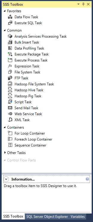
If we were working with the data flow, we would see a different set of components, but you don’t need to worry about that for now. We’ll get to the data flow in a bit. Just know that you need to have the SSIS Toolbox pane open before you can add those components to our package file. Before we do that, however, we’re going to first define a couple connection managers.

Adding connection managers

In SSIS, when you retrieve data from a source or load data into a destination, you must define a connection manager that provides the information necessary to make the connection. In this case, we need to create a connection manager for the EmployeeData.txt file and one for the AdventureWorks2014 database.

We don’t have to create the connection managers in advance; we can create them when adding components to the control flow or data flow. It’s mostly a matter of preference. Personally, I like to set up the connections as a separate step so I don’t have to mess with them when focusing on the other components.

To set up the connection managers, we can use the Connection Managers pane at the bottom of our design surface. Let’s start with the one for the AdventureWorks2014 database. Right-click an area within the Connection Managers pane, and then click New OLE DB Connection. In the Configure OLE DB Connection Manager dialog box, click New.

When the Connection Manager dialog box appears, provide the name of the SQL Server instance, select the authentication type (specifying a user name and password, if necessary), and then select the AdventureWorks2014 database, as shown in the following figure.

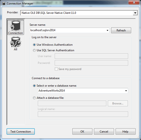
At this point, it’s a good idea to test your connection. If you run into problems here, you will certainly run into problems when you try to configure other components or run the package. If you test it now, you’ll at least rule out any immediate issues, assuming you can successfully connect to the database.

When you click OK, SSIS creates the connection manager and lists it in the Connection Managers pane. By default, the connection manager name includes both the SQL Server instance and database names. In this case, I shortened the name to include only the database component, just to keep things simple when I reference it later in the article. You can use whatever name best serves your purposes.

To change the name, right-click the connection manager in the Connection Managers pane, click Rename, and then edit the name.

Now let’s create the connection manager for the EmployeeData.txt file. Once again, right-click an area within the Connection Managers pane, but this time, click New Flat File Connection. When the Flat File C onnection Manager Editor dialog box appears, provide a name (I used EmployeeData.txt) and description. For the File name option, navigate to folder where you created the EmployeeData.txt file and select that file. The File name option should include the full path, as shown in the following figure.

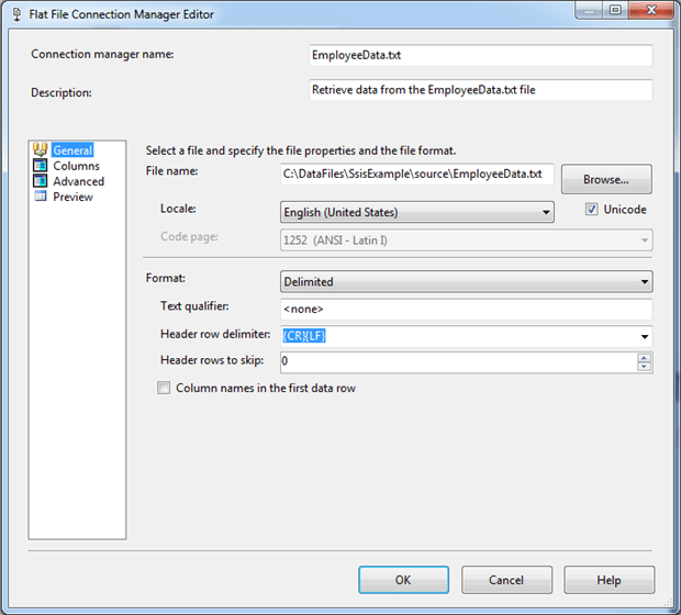
Note the Column names in the first data row option. This should not be selected because the source data does not include the column names. If it is selected, clear the check box.

That’s all there is to creating the two connection managers. We can now reference them within any our package components as we define our ETL operation.

Defining the control flow

When you open an SSIS package file in Visual Studio, you’re presented with a design surface that includes several tabs. By default, the designer opens to the Control Flow tab, which is where we define the package workflow. We have to start with the Control Flow tab, at least initially, before we can define the data flow, the core of the ETL operation.

SSIS provides the building blocks we need to define the control flow. They come in the form of tasks and containers that we drag from the SSIS Toolbox pane to the control flow design surface. A task is a component that performs a specific function, such as run a T-SQL statement or send an email message. A container provides a structure for organizing a set of tasks into isolated actions, such as implementing looping logic.

For this article, we will build a control flow that can be broken down into the following steps:

1. Truncate the EmpSales and EmpNonSales tables so they contain no data when we insert the new data.
2. Provide a structure (referred to as the data flow) for carrying out the actual ETL operation.
3. Archive the the EmployeeData.txt file after the data has been loaded into the target tables.

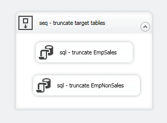
For the first step, we’ll add a Sequence container to the control flow and then add two Execute SQL tasks to the container. The Sequence container provides a simple means for grouping tasks together so they can be treated as a unit. Although it’s not necessary to use the container, adding it will give you a general sense of how containers work.

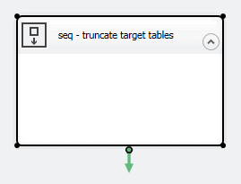
To add the container, drag it from the SSIS Toolbox pane to the design surface and change the name to seq – truncate target tables. To rename the component, right-click the container, click Rename, and then type in the new name.

You can name a component anything you like, but it’s generally considered a best practice to provide a name that briefly shows what type of component it is and then describes what it does. In this case, I’ve used a three-letter code ( seq) to represent the Sequence container, but you can use whatever system works for you. In the end, you should have a component on your design surface that looks similar to that shown in the following figure.

Next, drag the Execute SQL task from the SSIS Toolbox pane to within the Sequence container on the design surface, and then double-click the component to open the Execute SQL Task Editor dialog box. Here you can provide a name-I used s q l – truncate EmpSales-and a description, as shown in the following figure.

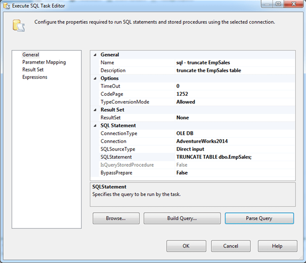
Next, select AdventureWorks2014 for the Connection property. This is one of the connection managers we defined earlier. Then, for the SQLStatement property, add the following T-SQL statement:

If you want to check whether your statement can be properly parsed, first change the BypassPrepare property to False, and then click Parse Query. You should receive a message indicating that the statement will parse correctly. Although this does not necessarily mean your statement will run when you execute the package, it does indicate that you probably got the syntax correct.

Now repeat these steps to add and configure an Execute SQL task for the EmpNonSales table. When you’re finished, your Sequence container should contain two tasks and look similar to what is shown in the following figure.

One of the advantages of a Sequence container is that it provides an easy way to execute the tasks within the container without running the entire package. To try this out for yourself, right-click the container (without clicking either task), and then click Execute Container. The tasks and container should run successfully, as indicated by the green circles with white checkmarks, as shown in the following figure.

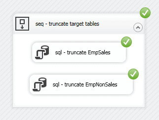
To return to the regular view of the control flow (and get out of execution mode), click the Stop Debugging button on the toolbar.

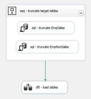
Now let’s move on to the second step of the control flow, which is to add a component that will carry out the actual ETL operation. Drag the Data Flow task from the SSIS Toolbox pane to the control flow design surface, beneath the Sequence container, and rename the task dft – load tables, or something like that.

Next, connect the precedence constraint from the Sequence container to the Data Flow task. A precedence constraint is a connector that links two components together to define the workflow. You can use precedence constraints to define the order in which the components run and under what conditions they’re executed. In this way, components run only when certain conditions are met.

A precedence constraint moves the workflow in only one direction. By default, the downstream component runs after the successful execution of the upstream component. If the upstream component fails, that part of the workflow is interrupted, and the downstream component does not run. However, you can configure a precedence constraint to run whether or not the upstream component fails or to run only if that component fails.

For this example, we’ll go with the default behavior, using a precedence constraint to specify that the Data Flow task should run after the Sequence container has been successfully executed. To connect the components, select the Sequence container so that it displays a green arrow at the bottom, and drag the arrow to the Data Flow task. When you release the mouse, a green directional line should connect the two components, as shown in the following figure.

For now, that’s all we’ll do with the Data Flow task. We’ll cover the task in more detail in the next section. Instead, let’s move onto the third step in the control flow, which is to archive our source file.

When archiving the file, we’ll move it to a different folder, renaming it in the process. To make this work we must first define a variable that adds the current date to the file name. To set up the variable, you should first open the V ariables pane if it is not already open. You can open the pane just like you did the SSIS Toolbox pane. Click the View menu, point to Other Windows, and then click Variables.

In the Variables pane, click the Add Variable button at the top of the pane. This adds a row to the grid where you can configure the variable’s properties. For the first four properties, use the following values:

• Name: path
• Scope: Package
• Data type: String
• Value: “”

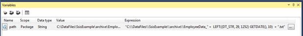
We need to specify only an empty string for the Value property because we’ll get the actual value by creating an expression. To create the expression, click the ellipses button associated with the Expression property. In the Expression Builder dialog box, type an expression in the Expression text box similar to the following:

The expression specifies the full path of the target folder, along with the first part of the file name, ending with an underscore. Notice we must enclose the string in double quotes and use a second backslash to escape each backslash in the path. Be sure to replace the path we’ve used here with one that works for your environment.

The expression then concatenates the path string with the current date, as returned by the GETDATE function. However, the function returns a full date/time value, but we want to use only the date portion. (Note that you can drag components from the upper two panes when building your expression.)

To extract the date, we must first convert the value to a string, using the DT_STR function, which precedes the GETDATE function. When calling the DT_STR function, we must include the function name, length of the string output, and the code page. In this case, we specify the length as 29 and the code page as 1252, which refers to the Latin-1 code page. This is the code page that is most commonly used.

We then enclose the date portion within the LEFT function, using the date expression as the function’s first argument and the number of characters (10, in this case) as the function’s second argument. The final part of the expression adds the .txt extension to the filename. The Expression Builder dialog box should now look similar to the one shown in the following figure.

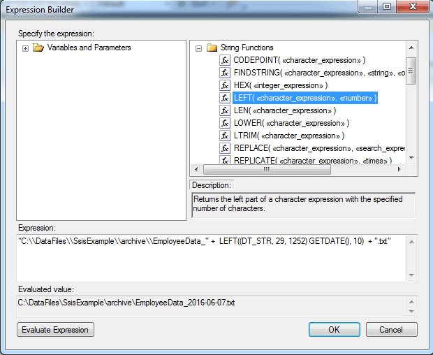
The Evaluated value section shows what the final variable value will look like, based on the current date. To get this value, you must click the Evaluate Expression button. If your expression is not correct, you will receive an error message, rather than an actual value.

After you finish creating the variable, the Variables pane should look similar to the one shown in the following figure. Depending on what other steps you might have taken within SSIS, the Value property might still show an empty string or show an actual value.

Now that we have our variable, we can do something with it. Drag the File System task from the SSIS Toolbox pane to the control flow, beneath the Data Flow task. Connect the precedence constraint from the Data Flow task to the File System task, and then double-click the File System task.

In the File System Task Editor dialog box, change the Name property to fst – archive file, and provide a description. For the Operation property, select Rename file from the drop-down list, and for the SourceConnection property, select the EmployeeData.txt connection manager.

Next, change the IsDestinationPathVariable property to True, and for the DestinationVariable property, select the path variable you just created. It will be listed as User::path, as shown in the following figure.

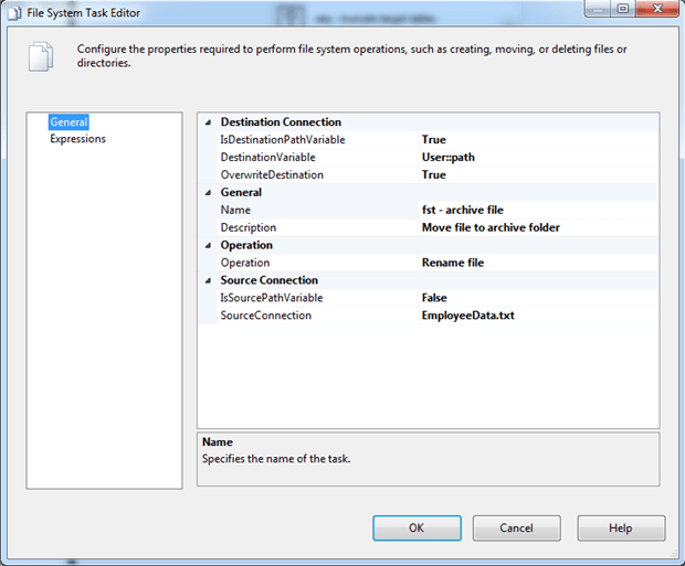
Notice that the OverwriteDestination property is set to True in the figure above. This can be handy when testing a package so you can easily re-execute the components as often as necessary, without having to manually remove the file or take other steps. In a production environment, you might want to select False for the property value

You’ll likely want to set up more complex naming logic for the archive file than what we’ve implemented in our solution, but what we’ve done here should be enough to demonstrate how the variable assignments work. That said, your control flow should now look similar to the one shown in the following figure.

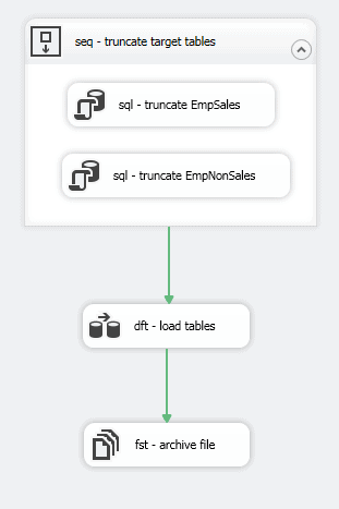
As you can see, we’ve defined all three steps of our control flow. We can even run the package to test that the control flow works. It won’t do much, other than archive the source file, but it will let you know if you’ve introduced any glitches so far.

To run the package, click the Start button on the toolbar. If all goes well, your results should look similar to what is shown in the following figure.

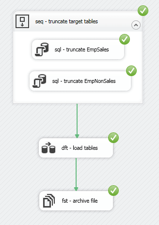
To return to the regular view of the control flow, click the Stop Debugging button on the toolbar. Keep in mind that, if you run the control flow, it will move and rename the file you created with the bcp command, in which case, you will have to rerun that command in order to continue on to the next set of examples.

Defining the data flow

Although our control flow includes the Data Flow task, the way in which we configure the task (and subsequently the data flow itself) is much different from the other control flow tasks. When you double-click the Data Flow task, Visual Studio takes you to the Data Flow tab, the second tab in the SSIS design surface, as shown in the following figure. There you add data flow components specific to the selected Data Flow task, much like you add components to the control flow.

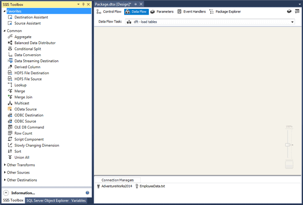
When you switch to the Data Flow tab, Visual Studio changes the components in the SSIS Toolbox pane to those specific to the data flow, with each component carrying out a specific ETL task. SSIS supports the following three types of data flow components:

• Source: A source component extracts data from a specified data source.
• Transformation : A transformation component transforms the data that has been extracted from a data source.
• D estination : A destination component loads the transformed data into a specified data destination.

SSIS provides a variety of components for each type in order to address different ETL needs. SSIS also allows you to incorporate custom components into your dataflow for addressing situations that the built-in components cannot support.

For the SSIS solution we’re creating in this article, the data flow will consist of the following seven steps, each of which is associated with a data flow component:

1. Retrieve the employee data from the EmployeeData.txt file.
2. Generate an alternate ID for each employee, based on the employee’s email address.
3. Convert the data type of the new column to one with a smaller size.
4. Split the data flow into two data groups: one for sales representatives, one for all other employees.
5. Look up the sales group associated with each sales rep.
6. Load the sales rep data in the EmpSales table.
7. Load the data for the other employees into the EmpNonSales table.

With this in mind, let’s get started with the first step by adding a Flat File Source component to the data flow. Drag the component from the SSIS Toolbox pane to the data flow design surface, rename it ffs – retrieve employee data, and double-click the component to configure it.

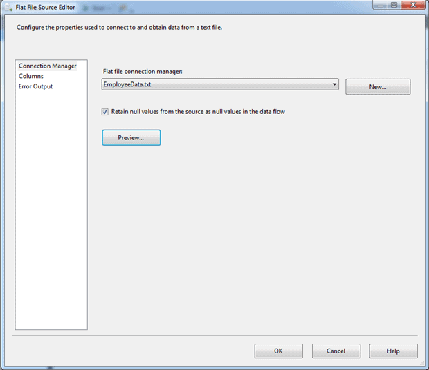
In the Flat File Source Editor dialog box, select the EmployeeData.txt connection manager from the drop-down list, and then select the option Retain null values from the source as null values in the data flow, if it is not already selected, as shown in the following figure.

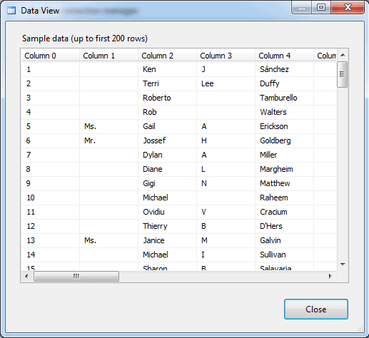
That’s all we need to do for the moment, but before you click OK, it’s always a good idea to preview the data to make certain you’re getting the results you want. To do so, click the Preview button. The Data View dialog box appears and provides a sample of the data, as shown in the following figure.

After you’ve previewed the data, click Close and then click OK to close the the Flat File Source Editor dialog box. Now we need to do some advanced configuring to make it easier to work with the prepared data in the downstream components.

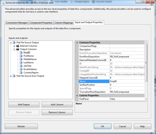
Right-click the Flat File Source component, and then click Show A dvanced Editor. In the Advanc ed Editor dialog box, go to the Input and Output Properties tab, and expand the Output Columns node in the Inputs and outputs pane.

Because the source data includes no column names, each column is assigned a generic name, starting with Column 0, Column 1, Column 2, and so on. For each column, you will either rename it or delete it:

• To rename a column, select the column and then update the Name property in the right pane.
• To delete a column, select the column and click Remove Column.

The following list shows which columns to rename, what names to use, or whether to delete the columns:

• Column 0: Rename to EmpID.
• Column 1 : Delete.
• Column 2 : Rename to FirstName.
• Column 3 : Rename to MiddleName.
• Column 4 : Rename to LastName.
• Column 5: Delete.
• Column 6 : Rename to JobTitle.
• Column 7 : Delete.
• Column 8 : Delete.
• Column 9 : Rename to EmailAddress.
• Column 10 : Delete.
• Column 11 : Delete.
• Column 12 : Delete.
• Column 13 : Delete.
• Column 14 : Delete.
• Column 15 : Delete.
• Column 16 : Rename to CountryRegion.
• Column 17 : Delete.

After you’ve finished renaming and deleting columns, your Input and Output Properties tab should look like the one shown in the following figure.

Next we will add a Derived Column Transformation component to generate a new column that contains the employee alternate ID, based on the first part of the email address.

To create the column, drag the Derived Column Transformation component onto the design surface, change its name to drv – generate EmpAltID, and connect the green connector from the Flat File Source component to the Derived Column Transformation component.

Although the connectors used in the data flow appear similar to those in the control flow, they are very different, which is why they’re referred to as data paths, rather than precedence constraints. Each data path represents a section of the pipeline as data moves through the ETL process. Data path behavior can vary from component to component, depending on the component type.

When we connect the data path from the Flat File Source component to the Derived Column Transformation component, we’re directing the data flow from the source component’s output to the transformation component’s input. We must establish this connection between the two components before we can properly configure the second component because it relies on the metadata from the first component, as it is presented via the data path.

After you connect the data path between the two components, double click the Derived Column Transformation component. In the Derived Column Transformation Editor dialog box, you’ll be working in the first row of the grid in the lower pane. To start, assign the name EmpAltID to the Derived Column Name property, and for the Derived Column property, select the option add as new column from the drop-down list, if it is not already selected.

Next, add the following expression to the Expression property:

The expression uses the LEFT function to return the value that precedes the at ( @) symbol. The FINDSTRING function determines that exact location of the first occurrence of that symbol, subtracting 1 to account for the symbol itself. When you add the expression, SSIS automatically assigns the DT_WSTR data type, which is a Unicode string, as shown in the following figure.

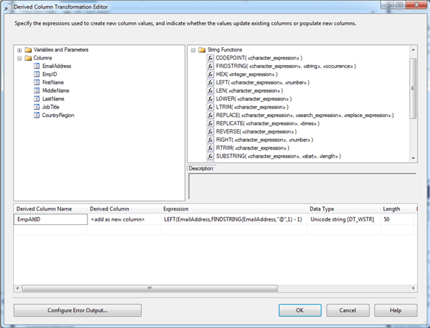
The component also assigns a size to the data type, based on the source data (in this case, the EmailAddress column). For the new column, we want to use the same data type, but reduce the size to 20, rather than 50. One way to do this is to update the expression to explicitly convert the output from the LEFT function, as in the following example:

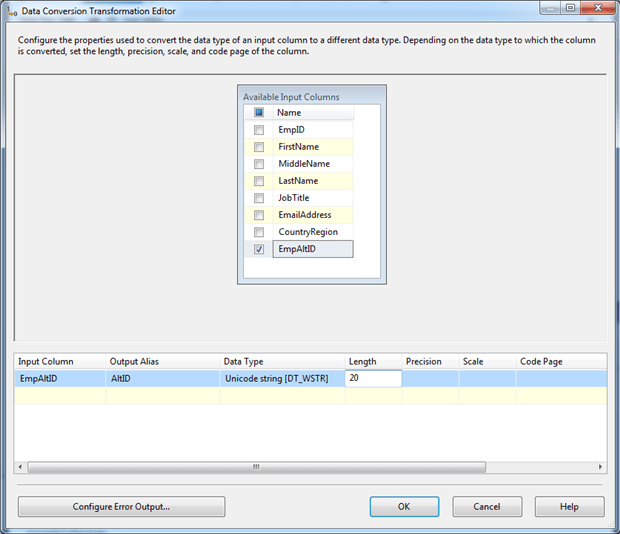
Another approach is to use a Data Conv ersion Transformation component to reduce the column size as a separate step. In this case, we’ll take this approach so we can demonstrate how the transformation works. You are likely to run into situations in which you must explicitly convert the data.

To make the change, add the Data Conversion Transformation component to the control flow, connect the data path from the the Derived Column Transformation component to the Data Conversion Transformation component, and change its name to cvt – trim EmpAltID.

Next, double-click the component to open the Data Conversion Transformation Editor dialog box, and then select the EmpAtlID column from the Available Input Columns box. Selecting the column adds a row to the grid in the bottom pane. In this row, change the Output Alias property to AltID, and change the Length property to 20. The dialog box should now look similar to the one shown in the following figure.

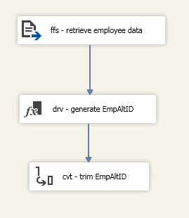
At this point, your data flow should include three components, one source and two transformations, with data paths connecting all three, as shown in the following figure.

The next step is to add a Conditional Split Transformation component to divide the data into two groups, one for sales reps and one for everyone else. To split the data, add the transformation to the data flow, connect the data path from the Data Conversion Transformation component to the Conditional Split Transformation component, and rename the component spl – separate sales staff.

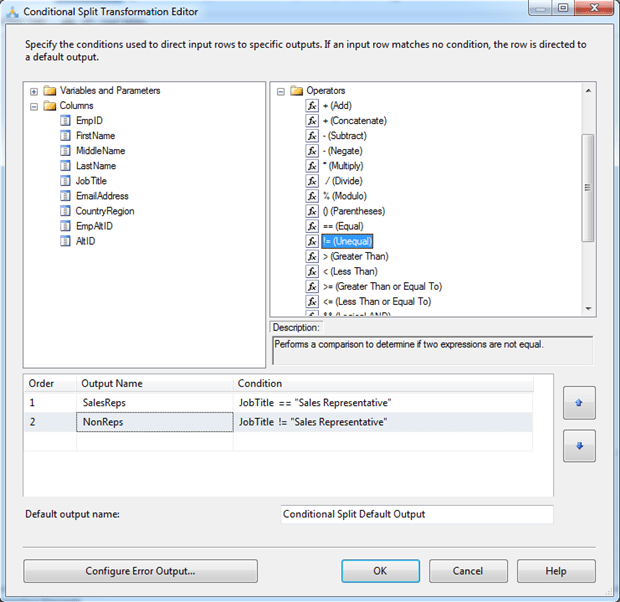
Next, double-click the component to open the Conditional Split Transformation Editor dialog box. Here we will create two outputs, one for each data group. To add the first output, click within the first row and change the Output Name property to SalesReps. Then add the following expression to the Condition property:

The expression states that the JobTitle value must equal Sales Representative for a row to be included in the SalesReps output.

Next, click in the second row and name the output NonReps. This time specify the following expression:

In this case, all rows whose JobTitle value does not equal Sales Representative are added to the NonReps output.

The Conditional Split Transformation Editor dialog box should now look like the one shown in the following figure.

Next, add a Lookup component to the data flow and rename it lkp – find sales group. We’ll use the transformation to look up the sales group for each sales rep. After you add and rename the component, connect the data path from the Conditional Split Transformation component to the Lookup component.

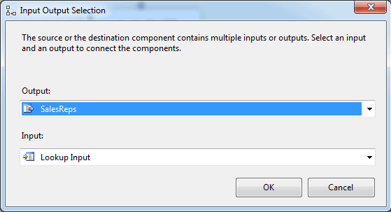
When you connect the components, the Input Output Select dialog appears. Here you select which output from the Conditional Split Transformation component to use for the Lookup component. In this case, we’ll use the SalesReps output, as shown in the following figure.

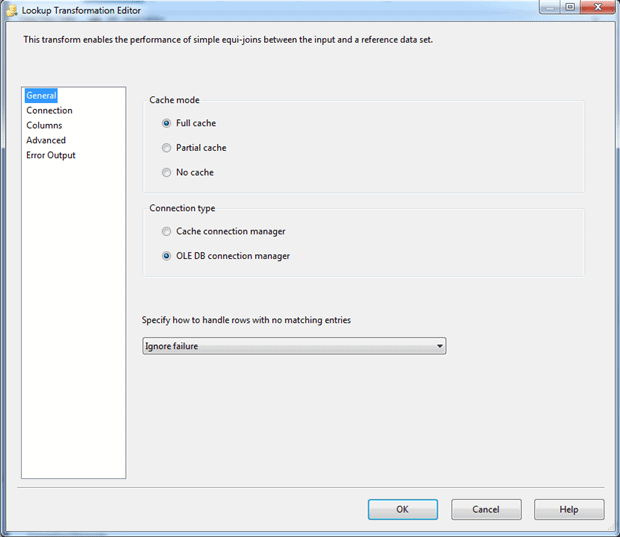
Next, double-click the Lookup component. In the Lookup Transformation Editor dialog box, ensure that the following three options on the General page are selected:

• Full cache : Uses an in-memory cache to store the reference dataset.
• OLE DB connection manager : Uses an OLE DB connection manager to connect to the source of the lookup date.
• Ignore Failure : Ignores any lookup failures, rather than failing the component or redirecting the row if no matches are found.

The following figure shows the General page with these three options selected.

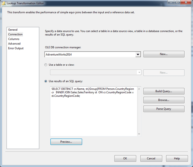
Now go to the Connection page. From the OLE DB connection manager drop-down list, select AdventueWorks2014, and then select the Use results of an SQL query option. Beneath the option, type or paste the following SELECT statement.

The statement joins the CountryRegion and SalesTerritory tables in order to retrieve the sales group associated with each country. In this way, we can retrieve the sales group for each sales rep, based on that rep’s country, which is part of the source data. After you add the SELECT statement, the Connection page should look similar to the following figure.

At this point, you might want to parse the query and preview the data to make sure everything is looking as you would expect.

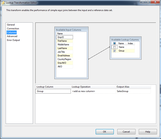
Next, go to the Column s page and drag the AltID column in the Available Input Columns box to the Name column in the Available Lookup Columns box. When you release the mouse, a line should connect the two columns (sort of).

Now select the Group column check box in the Available Lookup Columns box. This adds a row to the grid in the bottom pane. In that row, change the name of the Output Alias property to SalesGroup. The following figure shows the Columns page after I configured it on my system.

If everything has gone as planned, your data flow should now look something like the one shown in the following figure.

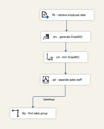
Next, add an OLE DB Destination component to the data flow and change the name to ole – load sales data. Connect the output data path from the Lookup component to the OLE DB Destination component. When the Input Output Selections dialog box appears, prompting you to choose an output, select the Lookup Match Output option.

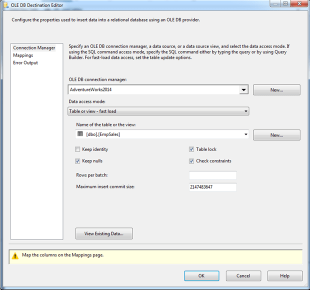
Now double-click the OLE DB Destination component. When the OLE DB Destination Editor dialog box appears, ensure that AdventureWorks2014 is selected as the connection manager and that EmpSales is selected as the target table, as shown in the following figure.

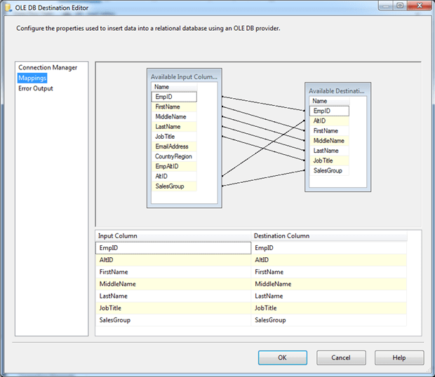
Next, go to the Mappings page and ensure that the columns are properly mapped between the available input columns and output columns, as shown in the following figure. SSIS should have picked up the mappings automatically, but you should make sure they’re correct.

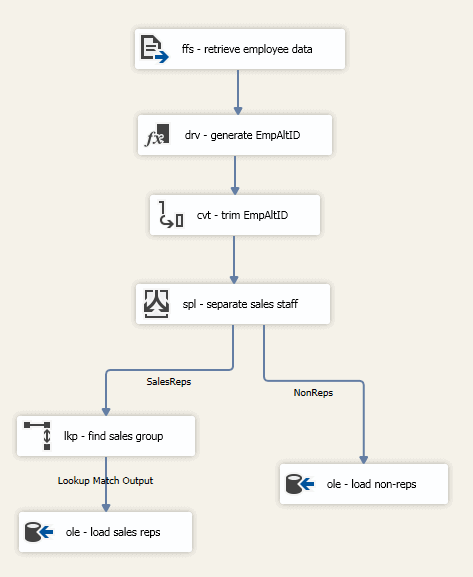
You now need to add a second OLE DB Destination component that connects from the Conditional Split Transformation component to the new destination. This time, use the NonReps output from the Conditional Split Transformation component and configure the OLE DB Destination component to load data into the EmpNonSales table. Your data flow should now look similar to the one in the following figure.

That should complete your data flow. You can now run the package to verify that everything is working as it should. Make sure you run the bcp command if necessary to generate your source file, if it no longer exists.

To run the package, click the Start button on the Visual Studio toolbar. If everything is working as it should, all the components will indicate that they have been successfully executed, as shown in the following figure.

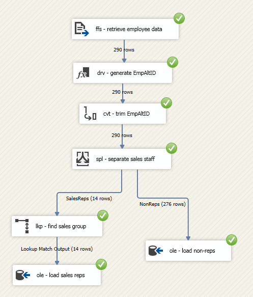
Notice that the execution results show the number of rows that passed through each data path as the data moved from one component to the next.

To return to the regular view of the data flow, click the Stop Debugging button on the toolbar.

Working with SSIS and SSDT

Although the SSIS package we developed here is a relatively basic one, it demonstrates many of the principles of how to build an SSIS solution. Of course, SSIS is able to do far more than what we’ve shown you here. Each component supports additional features, and there are many components we have not covered.

As you work with SSIS, be sure to refer to SQL Server documentation for specific information about SSIS and SSDT. If you were already using SSIS prior to the switch from BIDS to SSDT, the transition should not be too difficult. Many of the concepts and features work the same way.

What we have not touched upon is how to implement and manage an SSIS package. We’ll have to save that for another article. Just know that, before you can implement an SSIS package, you must have already developed that package and made sure you can run it. With luck, this article has provided the starting point you needed for developing that package and seeing for yourself how easily you can extract, transform, and load data.