“Prediction is very difficult, especially if it’s about the future.” – Niels Bohr

In this article we will look at predictive analytics, and try to explain its uses and how it works. After the introduction, we will dive into a brief example and some R code samples.

What is predictive analytics?

‘Predictive analytics’ is a term that refers to a variety of techniques for determining the probability of certain future events from the current and historical data. Generally, this is done by studying the interrelationships between many measurable factors to determine ‘risks’ or the ‘likelihood’ of an event happening. It has long been used to determine such essential commercial information as credit risk, potential fraud, and law enforcement. It is a well-established way to gauge the solvency of a commercial organization or the stability of currency.

Now that data-processing power is so cheap, the potential data is easy to get, and there are tools to do the statistical analysis, it has been feasible to extend the use of predictive analytics to marketing and routine business strategy for such purposes as predicting churn or estimating demand. It is already well-used in manufacturing to predict more exactly when components need to be ready at the assembly-line, and for large engineering projects to predict timescales.

What kinds of data are the predictive analytics based on?

Let’s take a short example of data in the retail sector:

• Descriptive data – these are the features of each user and they make it more or less unique
  • Attributes – names, taxpayer number, gender…
  • Self-declared information – interests, hobbies, religion…
  • Demographics – age, family status, household information…
• Behavioral data
  • Transactions / orders – bought items value, returned items, deleted items from the shopping cart…
  • Filters – what products were filtered and why…
• Interactional data
  • Call center notes – notes from interactions with customer support
  • Email correspondence – written correspondence with customer support
  • Web clicks – web browsing history, product pages viewed..
  • Search history – search history on the site, products searched for..
• Attitudinal data
  • Opinions – any web data from which an opinion can be derived
  • Preferences – any other web data from which individual preferences or needs can be derived
  • Survey results – for example, customer satisfaction surveys
  • Social media interactions – likes, comments and chats on social media are fruitful assets when it comes to discovering valuable information about individuals or groups (such as my Facebook picture showing me bungee jumping, and me wondering at the same time whether sharing this picture affects my medical insurance premium)

Some businesses are smarter than others in collecting this sort of data, buying it and analysing it to inform their strategy or promote sales. The more data there is and the better it is analyzed, the better and timelier decisions can be made to determine the direction of the business based on solid data rather than ‘gut feeling’ or intuition.

What is predictive analytics used for?

We can outline three different sectors in which the predictive analytics are very valuable:

• Customer analytics – in my previous article Getting to know your customers better – cohort analysis and RFM segmentation in R I mentioned some techniques and examples of customer segmentation and analysis of user behavior. The most important point to take out of this article was the need of several points / snapshots over time in order to detect customer intentions and segment movements. Another point I must make now, is that data analysis does not mean much unless an action is to be taken based on it.
  Also, the choice of communication channel is very important: if we are to do bare customer segmentation and RFM analysis, this takes a few weeks or months and if the only thing we do is to send emails to certain customer segments post factum, this seems like a terrible idea. Think about it this way: if, by doing some segmentation, we have detected that a group of customers have churned, it is already too late to email them and beg them to come back. Here is where predictive analytics comes in: by discovering patterns in historical data we can predict which customers may churn and when, and we can do real-time targeting and offers or discounts based on their preferences, shopping history and so on.
  • Acquire new customers
  • Grow and educate customers
  • Retain customers
  • Lose customers (recently a company increased their customer engagement by sending out a very simple email to customers which had churned; the email simply stated “Your account with us hasn’t been used recently, please close it”. Funnily enough, this re-engaged more than half of the churned customers!)

In general, not all customers have the same value for a business. Here are the basic actions a business can take on a customer:

It really depends on the business decisions, and it really depends on the phase the business is in, and sometimes acquiring new customers may be cheaper than retaining or growing customers. Retention is not about keeping every customer either: in reality it is about keeping the good paying customers and not about keeping every single one. And data can easily answer such questions.

Operational analytics – this type of analytics is relevant for the supply chain, manufacturing or the services industries. Predictive analytics can cut costs and help increase customer satisfaction by providing better services. Historical data can be mined and models can be created to try and predict the demand of products and services for a certain period of time, so that the business can adjust and prepare for the supply. Threat and fraud detection – this type of analytics covers a large area and it ranges from monitoring environments to detecting fraud or crime. For example, analyzing insurance claims and collecting data related to insurance claims can decrease the amount of fraudulent claims, which in its turn means savings for the business.

Building a Predictive model

There are three basic type of model used for predictive analytics: the Predictive model, Descriptive model and the Decision model. Predictive models aim to determine how an individual within a population is likely to behave in response to a change in one or more variables in context, Descriptive models aim to classify individuals into groups who have characteristics in common, and decision models are used to develop a set of effective business rules that can guide the best way of managing processes or catering for particular customers.

Any predictive model has to be constructed, and then tested with separate data.

The success of a predictive model depends on the data fed into it, and there is of course a computational balance between complexity and time. I.e. the more data we feed into the model – the more variables we use, but it may take longer to compute. Aside from the time-consumption, there are couple other issues which can make a model clumsy:

• Overfitting – it occurs when a model becomes excessively complex (by having too many parameters for few observations) and in such case the model ends up describing a random noise in the data instead of underlying dependencies in the data.
• the fact that we need to put work into collecting, cleansing and relating data from different sources just to make it reliable for modelling

How does it work?

Building a predictive model is fairly straightforward, though it involves several steps:

• Collect relevant data – for this we would use any ETL tool to collect, cleanse and relate data from different sources
• Split the dataset into two sets (training set and verification set)
• Apply an algorithm to the training set to create a set of rules which will be used to fill in the target variable (the variable we are trying to predict)
• Create a model which is based on the rules established by the algorithm during the training phase
• Test the model on the verification data set – the data is fed to the model and the predicted values are compared to the actual values and thus the model is tested for accuracy
• Use the model on new incoming data and take action based on the output of the model

Let’s get our hands dirty with some code

For the examples in this article we will be using the R language.

The predictive analysis is done in two stages:

• Training a model
• Applying the model

Many models can be used for doing the predictive analysis, but they can be generalized in two types:

• Classification – predicting a category: a value that is discrete, finite with no ordering
• Regression – predicting a numeric quantity: a value that is continuous and infinite with ordering

As a hands-on example, we will take two of the most popular algorithms in data analysis: Linear regression and neural network.

There are two datasets we will be using for this:

• The iris dataset for classification problems – the iris dataset contains petal and sepal lengths data for each of the 3 kinds of iris flowers. The dataset can be used to predict the classification of any other variables of petal and sepal length.
• The prestige dataset from the car package for regression problems – the Duncan’s Occupational Prestige Data contains occupation data for the US in the 1950s.

Let’s load the datasets:

This code is for the iris data:

This code is for the prestige data:

Linear regression

Linear regression is one of the most popular and extensively-explored methods for data exploration. The linear regression model assumes that the linear relationship exists between the input and the output variables.

Let’s dive in the example. Make sure that we have already run the code from above, which prepares our datasets:

As mentioned earlier in the article, we have one training dataset, which is used to train our model, and another dataset, which will be used to test the model.

In the code above, we use the which function to assign to the testidx variable every fourth item of the entire dataset, and then we use this testidx array to create the training and the test datasets (the prestige_train dataset is 3 times bigger than the prestige_test dataset).

Now that we have prepared the objects, let’s fit the model by using the following code:

This code uses the lm function to fit the model. There are many ways we can fit a model, i.e. there are many combinations of predictor variables we can use. In this case we are using the prestige~. as the formula, which means that all variables in the prestige_train dataset, except for the destination variable, are evaluated.

Now we’ll use the model to predict the output of the test dataset:

Now that we have fitted the model, we will see if it is any good. We can use the summary function for diving into the details of the model:

The function returns the following result:

This seems exciting, but what does it mean?

So, this is how we built a regression model to try and predict the prestige based on a small dataset. It turned out that the most relevant (reliable) variables affecting prestige would be education and income. Now that we have built our model and we know what to expect of its performance, we can apply it to a larger datasets.

Of course, it is harder to spot a bad model compared to picking a good one. The models should be tested extensively, and not only checked by the R-squared value. R includes many ways to check models and here are a few links for further reading:

• Advanced Interpretation of R models
• Residuals in R
• Multiple Regression in R

Neural network

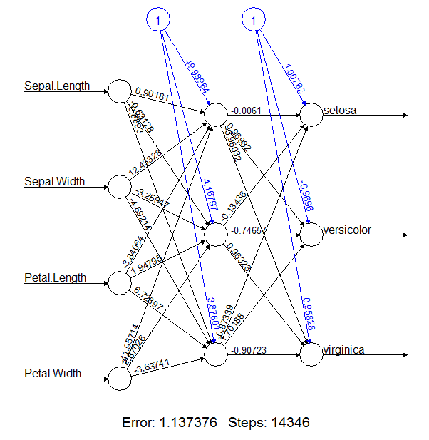
The idea behind a neural network resembles the human brain – a network of neurons that are interconnected. I.e. it is a set of computational units, which take a set of inputs and transfer the result to a predefined output. The computational units are ordered in layers, so they can connect the features of an input vector to the feature of an output vector.

The idea behind this is to train neural networks to model the relationships in the data.

Here is an example of a neural network model:

Lets dive into the example and prepare our datasets:

If we do not have the nnet package already installed, we can do this by using:

Lets load the nnet library and initialize our variable:

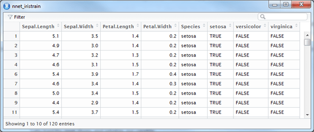
We now ‘binarize’ the categorical output of the training set, which means that we create three columns – one for each flower type – and set the bit flag according to the classification:

This will give us a dataset similar to this:

Now to fit the model:

And finally, we would make the predictions over the dataset:

In this case we are using the fitted model to predict the species of the iristest dataset and we are using the classification method.

Finally compare the accuracy:

Here we are comparing the array of the predicted output with the array of actual values in the Species of the iristest dataset.

The result is this table:

In this case the prediction was absolutely accurate, but this is not always the case with any of the methods for predictive analysis.

It is interesting to note the stochastic nature of the neural networks. This means that we should not expect the same result every time we run the algorithm. (After all, if neural networks were giving the same results every time, the humanity would have been unable to innovate!)

Let’s take an example of a different implementation of the neural networks with the neuralnet package:

The result we get is slightly different:

As we can see, two of the classifications are not matching the results. In reality, the models will perform differently, and this is quite normal. It is important for the predictive models to be tested and adjusted according to the constantly changing nature of the source data.

Summary:

In this article we have seen what predictive analytics are, how the mechanics behind them work and how they can be applied to solve classification and regression problems.

Before the hands on examples, we took a dive into what data can be used for the predictive analytics and what areas the analytics can be applied in. The most important point remains: data analysis is not worth anything unless it is acted upon as fast as possible.

We looked at two of the most popular algorithms for data analysis – Neural networks algorithm for classification and Linear regression for predicting numeric values. It is important to notice that in reality, different approaches and algorithms can be applied to solve the same challenge with the same dataset, however often they will give different results. No algorithms is universally optimal and this is why it is a good idea to test different approaches to the same dataset and compare the results.