
Recently, I was asked a couple of questions related to SQL Server statistics. The questions were:
- Should I care about the amount of statistics on my database?
- How much space does a statistics object use?
The distribution statistics of a column or an index are used by the Query Optimizer to judge the best strategy or plan for executing SQL statements. If the statistics are missing or out of date, then performance will suffer. I hope that I answered the two questions satisfactorily at the time, but they stuck in my mind because I’m addicted to query tuning and to understanding how the Query Optimizer works. I eventually decided to give them a fuller answer in this article.
Before answering the questions, I need to explain a few things about distribution statistics: what they are, why they’re important, and how they are created, updated, displayed and queried.
What are Distribution Statistics?
I couldn’t write about statistics without mentioning Holger Schmeling’s book ‘SQL Server Statistics’, so if, as you should, you want to know more about statistics, then I really recommend you to read it, since it is one of the most interesting books I’ve read; it is very cleanly written, he doesn’t waste time being verbose, you’ll know what you need to know, and that’s it.
Statistics, which contain a map or histogram of the way that data is distributed in a column or index, are there for the benefit of the Query Optimizer, to help it decide on the best query plan. When things are going well, you don’t have to worry too much about them. Generally, they are created automatically, and kept up-to-date as the data changes without any intervention. If the Query Optimizer is ‘compiling’ a query, and there aren’t any suitable statistics to determine how the data is distributed in the table or index, one is created at the point where it’s required, such as when you are using a column in a WHERE clause or when you are DISTINCTing a column.
So let’s take a look at the histogram that is in a statistics object. A histogram measures the frequency of occurrence for each distinct value in a data set. The Query Optimizer computes a histogram on the column values in the first key column of the statistics object. A histogram is a set of up to 200 values for a given column.
We can easily take a look at them. Here is a command to see the details about a specific statistic:
|
1 |
DBCC SHOW_STATISTICS (Tab1, Stats_MyStatOnCol1) |
Result:
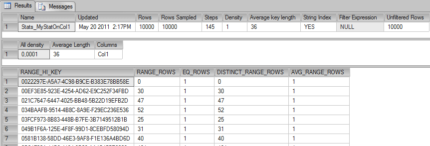
You’ll notice that three results are being returned, the header, the density vector, and the histogram.
The columns returned in the header contain a number of useful values (you can get this by querying DBCC SHOW_STATISTICS with STAT_HEADER specified). The attributes of the statistics object that are supplied in the header are:
| Name | Name of the statistics object. |
| Updated | Date and time the statistics were last updated. The STATS_DATE function is an alternate way to retrieve this information. |
| Rows | Total number of rows in the table or indexed view when the statistics were last updated. If the statistics are filtered or correspond to a filtered index, the number of rows might be less than the number of rows in the table. For more information, see Using Statistics to Improve Query Performance. |
| Rows Sampled | Total number of rows sampled for statistics calculations. If Rows Sampled < Rows, the displayed histogram and density results are estimates based on the sampled rows. |
| Steps | Number of steps in the histogram. Each step spans a range of column values followed by an upper bound column value. The histogram steps are defined on the first key column in the statistics. The maximum number of steps is 200. |
| Density | Calculated as 1 / distinct values for all values in the first key column of the statistics object, excluding the histogram boundary values. This Density value is not used by the Query Optimizer and is displayed for backward compatibility with versions before SQL Server 2008. |
| Average Key Length | Average number of bytes per value for all of the key columns in the statistics object. |
| String Index | Indicates the statistics object contains string summary statistics to improve the cardinality estimates for query predicates that use the LIKE operator; for example, WHERE ProductName LIKE ‘%Bike’. String summary statistics are stored separately from the histogram and are created on the first key column of the statistics object when it is of type char, varchar, nchar, nvarchar, varchar(max), nvarchar(max), text, or ntext. |
| Filter Expression | Predicate for the subset of table rows included in the statistics object. NULL = non-filtered statistics. For more information about filtered predicates, see Filtered Index Design Guidelines. For more information about filtered statistics, see Using Statistics to Improve Query Performance. |
| Unfiltered Rows | Total number of rows in the table before applying the filter expression. If Filter Expression is NULL, Unfiltered Rows is equal to Rows. |
There is also a density vector with these columns which we’re not going to elaborate on in this article.
| All Density | Density is 1 / distinct values. Results display density for each prefix of columns in the statistics object, one row per density. A distinct value is a distinct list of the column values per row and per columns prefix. For example, if the statistics object contains key columns (A, B, C), the results report the density of the distinct lists of values in each of these column prefixes: (A), (A,B), and (A, B, C). Using the prefix (A, B, C), each of these lists is a distinct value list: (3, 5, 6), (4, 4, 6), (4, 5, 6), (4, 5, 7). Using the prefix (A, B) the same column values have these distinct value lists: (3, 5), (4, 4), and (4, 5) |
| Average Length | Average length, in bytes, to store a list of the column values for the column prefix. For example, if the values in the list (3, 5, 6) each require 4 bytes the length is 12 bytes. |
| Columns | Names of columns in the prefix for which All density and Average length are displayed. |
As well as the header and density vector, there is a histogram that shows the distribution of data in the column. Here is a simple histogram of a table with an integer column:
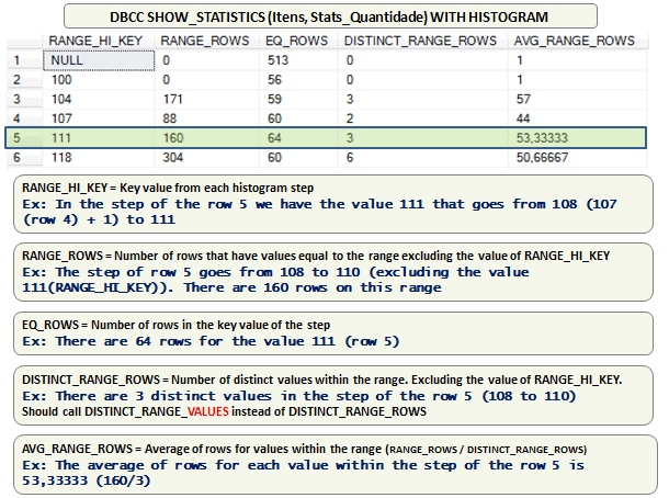
Figure 1: Histogram of the ‘itens’ table .
To illustrate the usage of a histogram, we’ll set up a very simple table, create some statistics on it, and see how the Query Optimizer is actually using the histogram. We’ll first create a table and then set up a statistics object with a histogram similar to the one in Figure 1. Here is a script to do it:
|
1 2 3 4 5 6 7 8 9 10 11 12 13 14 |
use tempdb GO IF OBJECT_ID('Itens') IS NOT NULL DROP TABLE Itens GO CREATE TABLE dbo.Itens(Quantidade int NULL) GO CREATE STATISTICS Stats_Quantidade ON Itens(Quantidade) GO UPDATE STATISTICS Itens WITH ROWCOUNT = 50000, PAGECOUNT = 180 GO UPDATE STATISTICS Itens Stats_Quantidade WITH STATS_STREAM = 0x01000000010... |
Because the hexadecimal representation that is used to set the Stats_Stream is too large, I’ve left out part of the code.
Now, let’s see the histogram of the table:
|
1 |
DBCC SHOW_STATISTICS (Itens, Stats_Quantidade) WITH HISTOGRAM |
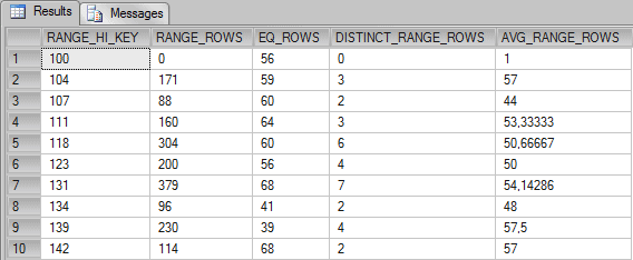
These columns have the following meaning, according to Books Online:
| RANGE_HI_KEY | Upper bound column value for a histogram step. The column value is also called a key value. |
| RANGE_ROWS | Estimated number of rows whose column value falls within a histogram step, excluding the upper bound. |
| EQ_ROWS | Estimated number of rows whose column value equals the upper bound of the histogram step. |
| DISTINCT_RANGE_ROWS | Estimated number of rows with a distinct column value within a histogram step, excluding the upper bound. |
| AVG_RANGE_ROWS | Average number of rows with duplicate column values within a histogram step, excluding the upper bound (RANGE_ROWS / DISTINCT_RANGE_ROWS for DISTINCT_RANGE_ROWS > 0). |
Example 1: (EQ_ROWS):
Let’s suppose that we want to execute the following query:
|
1 2 3 |
SELECT * FROM Itens WHERE Quantidade = 107 OPTION (RECOMPILE) |
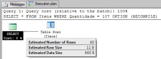
As we can see, SQL Server estimated that 60 rows will be returned for the value used in the WHERE clause – 107. This number is the value on the column EQ_ROWS for the histogram step 107 in the row 3.
Example 2: (RANGE_ROWS + EQ_ROWS):
Now, what if we execute this query?
|
1 2 3 |
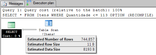
SELECT * FROM Itens WHERE Quantidade <= 107 OPTION (RECOMPILE) |
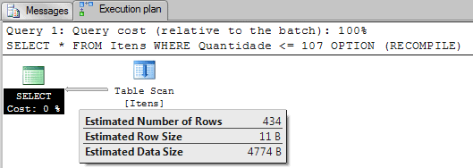
Now, because we are filtering using “Quantidade <= 107” the Query Optimizer sums the number of rows in the histogram that represents this formula.
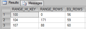
0 + 56 + 171 + 59 + 88 + 60 = 434
Example 3: (AVG_RANGE_ROWS):
Now, let’s suppose that we run the following query:
|
1 2 3 |
SELECT * FROM Itens WHERE Quantidade = 108 OPTION (RECOMPILE) |
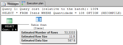
Now, because we are filtering by a value that is not in the histogram, the Query Optimizer uses the column AVG_RANGE_ROWS to estimate how many rows will be returned. The 53,3333 is the average of rows for values between 108 and 110.
Example 4: (RANGE_ROWS + EQ_ROWS + AVG_RANGE_ROWS):
Now, let’s consider the execution plan from running the following query:
|
1 2 3 |
SELECT * FROM Itens WHERE Quantidade <= 112 OPTION (RECOMPILE) |
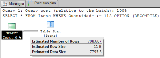
This example is similar to Example 2, where SQL Server has to sum all values to estimate the number of rows, the difference is that the value 112 is not on the histogram. Because of that, the value of avg_range_rows (50.66667) is added to the sum once for this missing value. That means:
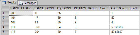
0 + 56 + 171 + 59 + 88 + 60 + 160 + 64 + 50.66667 = 708.66667
Example 5: (RANGE_ROWS + EQ_ROWS + SPECIAL_AVG_RANGE_ROWS ):
Now let’s look at this query:
|
1 2 3 |
SELECT * FROM Itens WHERE Quantidade <= 113 OPTION (RECOMPILE) |
This query is very similar to the query in Example 4. The difference is that instead of querying for 112, I’m now querying for “Quantidade <= 113”. You may expect that this is easy for the Query Optimizer, it’s just a matter of using the avg_range_rows to add the missing values, in this case adding 50.66667 twice.
If you add 50.66667 twice for the missing values (112 and 113 are not on histogram) you’ll have the following formula:
0 + 56 + 171 + 59 + 88 + 60 + 160 + 64 + 50.66667 + 50.66667 = 759.33334
As you can see, the value estimated by Query Optimizer was 744,857. So the question is, ‘How did the Query Optimizer get this number?’
The answer is, it added 43.42857 twice instead. Now the subsequent question is, ‘How did the Query Optimizer get this number?’
The answer is this. Instead of using the column avg_range_rows, it uses a new formula, that is, special_avg_range_rows = range_rows / (distinct_range_rows + 1). If you do it with the data in line 5 for the histogram you will have the value 43.42857.
304 / (6+1) = 43.42857
Our final formula to get the estimate number of rows is:
0 + 56 + 171 + 59 + 88 + 60 + 160 + 64 + 43.42857 + 43.42857 = 744.85714
I do not agree with this strategy for the “new” column. In my tests, if I use the avg_range_rows as the base for estimating my queries, I get a better number than the Query Optimizer’s estimation. I’m sure there is a reason behind this technique, maybe the data I tried was not the right data to test this.
You may be asking yourself a few questions on seeing this. If I’ve guessed what they are, here are the answers:
- Is this a bug? No, it’s the way it works.
- Is this perfect? No, and this is not supposed to be perfect anyway.
- Is this always a problem? No.
- Can this be a problem? Yes.
- Can we “fix” this? No.
By the way, the name “special_avg_range_rows” doesn’t exist outside this article. I invented the name to make things clearer. OK?
Example 6: (SPECIAL_AVG_RANGE_ROWS – WRONG ESTIMATION?):
Now we will test another query:
|
1 2 3 |
SELECT * FROM Itens WHERE Quantidade BETWEEN 112 AND 117 OPTION (RECOMPILE) |
As we can see, we are now applying a filter to return all rows where “Quantidade is between 112 and 117”. We already have the number of rows that satisfy this query on the Statistics Histogram. This is line 5 of the RANGE_ROWS column in the histogram, which means 304 rows will be returned. In the RANGE_ROWS column for the histogram, step 118 (row 5), we have all values that goes from 112 to 117, but SQL Server estimated the number of rows using another formula I haven’t yet fathomed. If you can work it out, please tell me.
Let’s just trust the histogram and the way that the Query Optimizer estimates the RANGE_ROWS. At least we’ve got a bit of an insight into the workings of the system.
Querying Statistics
Now we have shown what the histogram looks like and seen roughly how it is working, the next important thing we need to know is how to query how many statistics a table has. We can achieve this with the following command:
|
1 2 3 4 5 6 7 8 9 10 11 12 13 14 15 16 17 18 |
SELECT Schema_name(sys.objects.schema_id) + '.' + Object_Name(sys.stats.object_id) AS Table_Name, sys.columns.name AS Column_Name, sys.stats.Name AS Stats_Name FROM sys.stats INNER JOIN sys.stats_columns ON stats.object_id = stats_columns.object_id AND stats.stats_id = stats_columns.stats_id INNER JOIN sys.columns ON stats_columns.object_id = columns.object_id AND stats_columns.column_id = columns.column_id INNER JOIN sys.objects ON stats.object_id = objects.object_id LEFT OUTER JOIN sys.indexes ON sys.stats.Name = sys.indexes.Name WHERE sys.objects.type = 'U' AND sys.objects.name = 'Tab1' ORDER BY Table_Name GO |
Result:
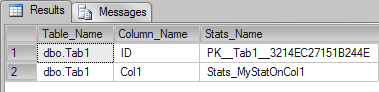
The command above is using the system tables to query the statistics that belong to a specific table.
Creating Statistics
Although the statistics objects you will see when you run this on your database are created automatically as required, you can create a statistics object manually using the following command:
|
1 |
CREATE STATISTICS Stats_MyStatOnCol1 ON Tab1(Col1) WITH FULLSCAN |
This command creates a statistics object on the column Col1 from the table Tab1. The command WITH FULLSCAN is an option to scan the entire table instead of just sampling it, so as to create a more accurate histogram for the statistic.
A full scan is more costly, but it is more accurate than a sampled scan.
Sampled Scan
By default, SQL Server can create or update statistics if it is able to recognize that the existing statistics object is outdated; I’ve described the algorithm for doing this in a note. When it detects that it doesn’t match the current data, SQL Server rebuilds the statistics using a SAMPLE of the data in the table. The default sampling rate is a slow-growing function of the table size, which allows statistics to be gathered relatively quickly even for very large tables.
When using sampling, SQL Server randomly selects pages from the table by following the IAM chain. Once a particular page has been selected, all the values from that page are used in the sample. This can occasionally lead to an unrepresentative sampling of data, in which case you may need to rebuild the statistics using the FULLSCAN option.
Note: You can read more about IAM Chains here: http://www.sqlskills.com/blogs/paul/post/Inside-the-Storage-Engine-IAM-pages-IAM-chains-and-allocation-units.aspx Note: Using the following information, you can check the formula used to “mark” statistics as outdated: Every time a column which belongs to a statistic receives sufficient modifications, SQL Server starts ‘Auto-Update Statistics’ to keep the data current. This works like so:
- If the cardinality of a table is less than six and the table is in the tempdb database, auto update after every six modifications to the table.
- If the cardinality of a table is greater than six, but less than or equal to 500, update statistics after every 500 modifications.
- If the cardinality of a table is greater than 500, update statistics when (500 + 20 percent of the table) changes have occurred.
- For table variables, a cardinality change does not trigger an auto-update of the statistics.
Full Scan
Some tables see frequent changes in the values in certain columns. Normally, statistics are then updated satisfactorily without you knowing, but if you notice that the sampled data used to create the statistics is not giving an accurate-enough representation, you can manually run an UPDATE STATISTICS with FULLSCAN using the following command:
|
1 |
UPDATE STATISTICS Tab1 Stats_MyStatOnCol1 WITH FULLSCAN |
Should I care about the amount of statistics on my database?
Usually I don’t need to care about the amount of statistics on my database, and the space they’re taking up, but not always. If you are dealing with a table that is very wide (many columns), then perhaps you should investigate whether the server is spending more time or resources in updating all these statistics than is really necessary.
I’ve already described how the DBCC DBREINDEX (<table>) of a table automatically triggers the update of ALL statistics for your table. That means that, if the statistics are never used, then you are wasting time and resources doing nothing.
If I have a very small maintenance window to rebuild my indexes and to update my statistics, I will probably remove all unused statistics of the bigger tables in the system in order to speed-up my rebuilds and statistics updates.
The problem with this strategy is that there isn’t any documented way to check if a statistics object is being used by a compilation, and I don’t yet know the undocumented way; it’s very hard to identify those statistics that are unused.
A very good way to start, as my friend Grant Fritchey reminded me, is to look at the duplicated statistics, by which I mean statistics auto created by SQL Server_WA_*, as you may already have created an index on this column. These statistics are not ‘auto-dropped’ when you create an index.
Testing
To show this in practice with a wide table, I created a script with a table called Tab1 with 10 thousand rows and 26 columns.
Here’s the script to create the table:
|
1 2 3 4 5 6 7 8 9 10 11 12 13 14 15 16 17 18 19 20 21 22 23 24 25 26 27 28 29 30 31 32 |
DROP TABLE Tab1 GO CREATE TABLE Tab1 (ID Int IDENTITY(1,1) PRIMARY KEY, Col1 VarChar(200) DEFAULT NEWID(), Col2 VarChar(200) DEFAULT NEWID(), Col3 VarChar(200) DEFAULT NEWID(), Col4 VarChar(200) DEFAULT NEWID(), Col5 VarChar(200) DEFAULT NEWID(), Col6 VarChar(200) DEFAULT NEWID(), Col7 VarChar(200) DEFAULT NEWID(), Col8 VarChar(200) DEFAULT NEWID(), Col9 VarChar(200) DEFAULT NEWID(), Col10 VarChar(200) DEFAULT NEWID(), Col11 VarChar(200) DEFAULT NEWID(), Col12 VarChar(200) DEFAULT NEWID(), Col13 VarChar(200) DEFAULT NEWID(), Col14 VarChar(200) DEFAULT NEWID(), Col15 VarChar(200) DEFAULT NEWID(), Col16 VarChar(200) DEFAULT NEWID(), Col17 VarChar(200) DEFAULT NEWID(), Col18 VarChar(200) DEFAULT NEWID(), Col19 VarChar(200) DEFAULT NEWID(), Col20 VarChar(200) DEFAULT NEWID(), Col21 VarChar(200) DEFAULT NEWID(), Col22 VarChar(200) DEFAULT NEWID(), Col23 VarChar(200) DEFAULT NEWID(), Col24 VarChar(200) DEFAULT NEWID(), Col25 VarChar(200) DEFAULT NEWID()) GO INSERT INTO Tab1 DEFAULT VALUES GO 10000 |
If I use DBCC to run a reindex on the table without creating any statistics, you’ll see something like this in the profiler:
|
1 2 |
DBCC DBREINDEX (Tab1) GO |
Now let’s suppose that you have created one statistics object for every column in the table. This means that the rebuild will fire the update of the statistics. This isn’t normally something you need to be concerned about, but you should know how to manage this.
To create one statistics object per column of the table I’ll run the procedure sp_createstats, which is documented in BOL.
Basically, this will create one statistics object per column for all tables in the database.
|
1 2 |
EXEC sp_createstats; GO |
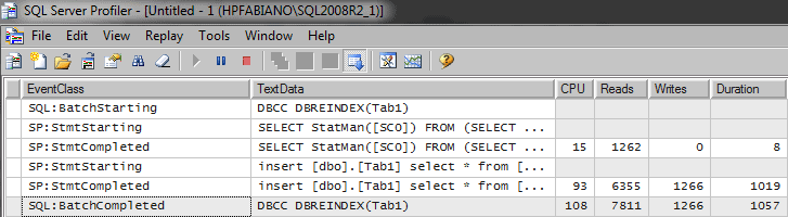
If, after running sp_createstats, I then rebuild the table, I’ll see something like this in the profiler:
|
1 2 |
DBCC DBREINDEX (Tab1) GO |
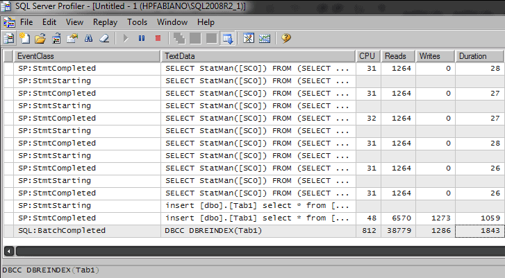
As we can see now we have a lot of update statistics (SELECT StatsMan…) running.
How much space can a statistics object use?
I don’t think you should be too concerned about the size and the quantity of statistics objects in your database. The space used by a statistics object is very small and isn’t something that will impact performance.
If you are a Doubting Thomas (like me) and need to verify this by seeing how much space is actually used, here we go.
In SQL Server 2000 this was easy, because the header, vector, and histogram were stored in the column statblob on the table sysindexes. A query on this table could answer how much space a statistics objects was using.
If we run a query on the NorthWind database in SQL Server 2000 we get something like the following:
|
1 2 3 4 5 6 7 8 9 |
-- Script to SQL Server 2000 SELECT LastTimeUpdated = STATS_DATE(si.id, si.indid), TableName = object_name(si.id), Name = RTRIM(si.name), [Size KB] = DATALENGTH(si.statblob) / 1024. FROM sysindexes si WITH (nolock) WHERE OBJECTPROPERTY(si.id, N'IsUserTable') = 1 AND STATS_DATE(si.id, si.indid) IS NOT NULL GO |
Results:
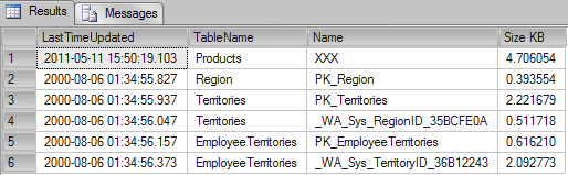
In the column Size KB we can see the KB each statistics object is using. Usually the size of the statistics object is around 8 KB of data.
In SQL Server 2005, and later versions, SQL Server started to store a distribution of the String values on the statistics. This information is also called “String Summary”, and this data can use more bytes.
The problem with checking the amount of space in the statsblob is that since SQL Server 2005, the column sysindexes.statblob returns NULL. Instead of doing this, we need to check the stats stream by using the DBCC SHOW_STATISTICS WITH STATS_STREAM command. Knowing this, we can build a script to execute the DBCC for each statistics object, store this in a temporary table, and then check the amount of bytes used by each statistics object.
The script looks like the following:
|
1 2 3 4 5 6 7 8 9 10 11 12 13 14 15 16 17 18 19 20 21 22 23 24 25 26 27 28 29 30 31 32 33 34 35 36 37 38 39 40 41 42 43 44 45 46 47 48 49 50 51 52 53 54 55 56 57 58 59 60 61 62 63 64 65 66 67 68 69 70 71 72 73 74 75 76 77 78 79 80 81 82 83 84 |
USE AdventureWorks GO IF OBJECT_ID('tempdb.dbo.#TMP') IS NOT NULL DROP TABLE #TMP GO CREATE TABLE #TMP (ID Int Identity(1,1) PRIMARY KEY, Table_Name VarChar(200), Column_Name VarChar(200), Stats_Name VarChar(200), ColStats_Stream VarBinary(MAX), ColRows BigInt, ColData_Pages BigInt) GO DECLARE @Tab TABLE (ROWID Int IDENTITY(1,1) PRIMARY KEY, Table_Name VarChar(200), Column_Name VarChar(200), Stats_Name VarChar(200)) DECLARE @i Int = 0, @Table_Name VarChar(200) = '', @Column_Name VarChar(200) = '', @Stats_Name VarChar(200) = '' INSERT INTO @Tab (Table_Name, Column_Name, Stats_Name) SELECT Schema_name(sys.objects.schema_id) + '.' + Object_Name(sys.stats.object_id) AS Table_Name, sys.columns.name AS Column_Name, sys.stats.Name AS Stats_Name FROM sys.stats INNER JOIN sys.stats_columns ON stats.object_id = stats_columns.object_id AND stats.stats_id = stats_columns.stats_id INNER JOIN sys.columns ON stats_columns.object_id = columns.object_id AND stats_columns.column_id = columns.column_id INNER JOIN sys.objects ON stats.object_id = objects.object_id LEFT OUTER JOIN sys.indexes ON sys.stats.Name = sys.indexes.Name WHERE sys.objects.type = 'U' ORDER BY Table_Name SELECT TOP 1 @i = ROWID, @Table_Name = Table_Name, @Column_Name = Column_Name, @Stats_Name = Stats_Name FROM @Tab WHERE ROWID > @I WHILE @@RowCount > 0 BEGIN --PRINT 'UPDATE STATISTICS "' + @Table_Name + '" "'+@Stats_Name+'" WITH FULLSCAN' --EXEC ('UPDATE STATISTICS "' + @Table_Name + '" "'+@Stats_Name+'" WITH FULLSCAN') INSERT INTO #TMP(ColStats_Stream, ColRows, ColData_Pages) EXEC ('DBCC SHOW_STATISTICS ("' + @Table_Name + '", "'+@Stats_Name+'") WITH STATS_STREAM') ;WITH CTE_Temp AS (SELECT TOP (@@RowCount) * FROM #TMP ORDER BY ID DESC) UPDATE CTE_Temp SET Table_Name = @Table_Name, Column_Name = @Column_Name, Stats_Name = @Stats_Name SELECT TOP 1 @i = ROWID, @Table_Name = Table_Name, @Column_Name = Column_Name, @Stats_Name = Stats_Name FROM @Tab WHERE ROWID > @I END GO SELECT SUM(DATALENGTH(ColStats_Stream) / 1024.) AS [Size KB] FROM #TMP GO SELECT Table_Name, Column_Name, Stats_Name, ColStats_Stream, DATALENGTH(ColStats_Stream) / 1024. AS [Size KB] FROM #TMP ORDER BY [Size KB] DESC |
Results:
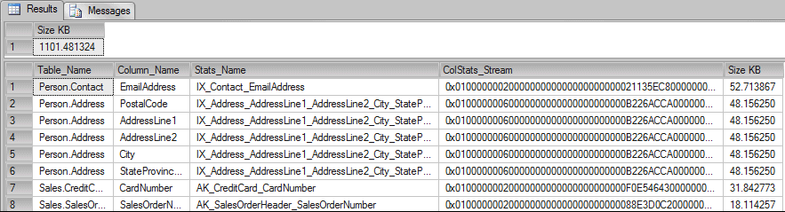
Now we can see that some statistics can use more space, but also, we can see that ALL statistics in the AdventureWorks database only use 1MB of data.
Note: Some undocumented code like stats_stream used in this article should be used with caution and not used in production environment.
That’s all folks, see you soon in the next article with more info about statistics
Load comments