
My crystal ball seems to be working again: The new addition to SQL Server 2019, shortest_path, was the subject of many of the technical sessions I delivered as one of the missing features of SQL Server Graph Database.
I will use an example that is similar to the first article I wrote on this topic. You can create the database and tables needed for this article using this script. Maybe you would also like to read the previous blog post about some recent improvements in Graph Databases.
Since the data is essentially a graph, a solution to visually show the results is helpful. An application like Gephi to can be used to view the graph. (You can download this application here.) To use Gephi with SQL Server, make sure that the TCP/IP protocol and mixed authentication are enabled. The app only supports SQL authentication, so you will need a SQL Server login to connect.
Using Gephi
Follow these steps to view the graph in Gephi.
- After opening Gephi, select New Project on the Welcome screen
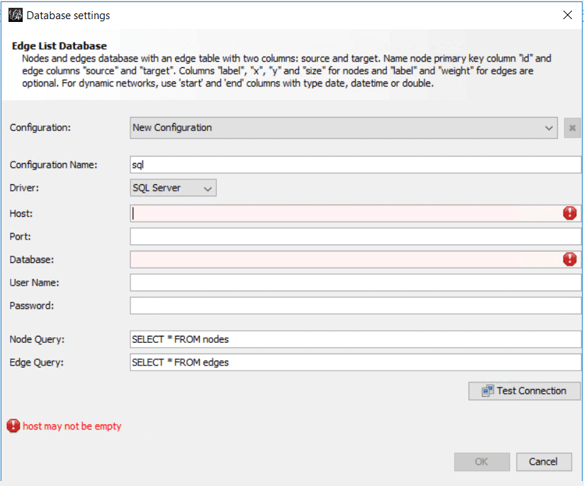
- On the File menu, select Import Database->Edge List. This will open the Database settings screen.
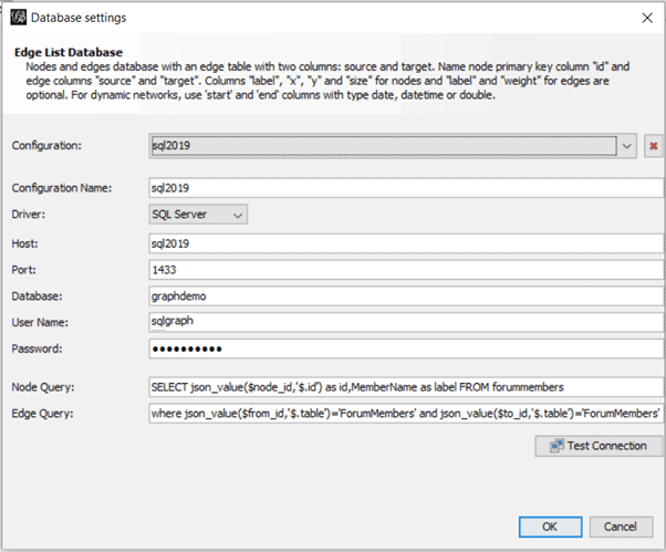
- In the Configuration Name field, create a name for the configuration, such as SQLServer2019.
- In the Driver field, select SQL Server.
- In the Host field, insert the machine/instance name of your SQL Server
- In the Port field, enter the port used, typically 1433. If you’re not sure, look for the port number in the SQL Server Configuration Manager program.
- In the Database field, insert the name of the database which contains the graph tables which is probably GraphDemo if you have been following along
- In the Username field, enter the username of a SQL Server login with SELECT permission to the tables in the GraphDemo database.
- In the Password field, insert the password for the SQL login.
In addition to the configuration required to connect to SQL Server, the Database settings screen also requires two queries: One to retrieve the list of nodes from the server and another to retrieve the list of edges from the server. I’ll explain those queries next.
The screen itself contains information at the top of the dialog about the columns the queries need to return, and it’s important to notice these columns are case sensitive.
The nodes table in SQL Server has the pseudo-column $node_id, which is a JSON column. A good option is to extract the id from the JSON and use the MemberName as the label for the node. The query will look like this:
|
1 2 3 |
SELECT Json_value($node_id, '$.id') AS id, membername AS label FROM forummembers |
The edge query has also to extract the id from $to_node and $from_node, but besides that, you need to filter the nodes returned, because the nodes table from the previous article has a relation between two members and between members and messages. For this example, return only the relation between two members. Here is the query:
|
1 2 3 4 5 |
SELECT Json_value($from_id, '$.id') AS source, Json_value($to_id, '$.id') AS target FROM likes WHERE Json_value($from_id, '$.table') = 'ForumMembers' AND Json_value($to_id, '$.table') = 'ForumMembers' |
It’s important to note that the source and target id’s in the edge query need to match with the ids in the node query. There are some additional columns that could be used, but for this example, you’ll only need these.
The final configuration will look similar to the following image:
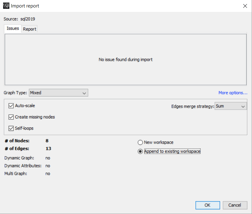
After you click OK, the next window, Import Report, involves many details but they will not be covered in this article. What’s important here is the number of nodes and edges found, confirming that the queries are correct. However, there is only a single step to be done on this screen:
Select the option Append to existing workspace.
After this first screen, you will see the Workspace1 and Preview tabs and Preview Settings window. It’s time to build the graph.
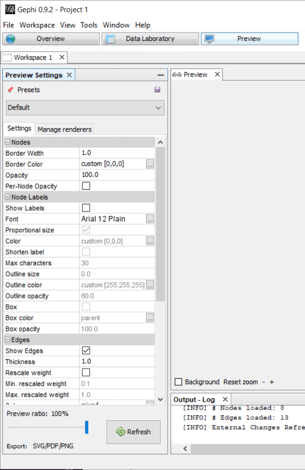
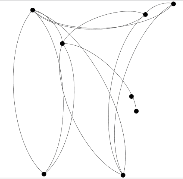
Click on the Refresh button inside the Preview Settings pane. This will result in an image similar to the one below. Note that yours may look different, but in the next step, you can verify that the nodes are connected correctly.
Improve this graph just a bit by making these changes in the Preview Settings tab.
- Change the Opacity property to 0 under Nodes.
- Mark the Show Labels property under Node Labels.
- Change the Outline opacity under Node Labels to 0
After clicking refresh, the graph will change to something like the image below:
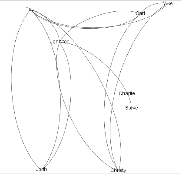
As you may notice, even a simple graph with a small amount of data can be quite complex to identify information such as the shortest path between two nodes in the graph. That’s why you need a tool to calculate this, and SQL Server 2019 can make this kind of calculation.
Calculating the Path
When you think about a function to calculate the shortest path between two points, you may think that it will be a simple function. To make this calculation work, however, you need way more than a simple function. You must establish paths among the graph data. The data has many paths, and each one has many nodes with a beginning and an end. Each path is a group of nodes, in some ways like the group by function.
One similarity, for example, is that you can’t read the column directly from the path. You need to apply aggregation functions to the set of nodes that are part of the path to read the information.
The syntax to build this query resembles the GROUP BY clause, requiring you to use aggregate functions to make calculations on every (shortest) path of nodes, getting grouped results.
To make this simpler, start to build the query over the model piece by piece. First, the From clause
|
1 2 3 4 |
FROM ForumMembers P1, ForumMembers FOR PATH as P2, Likes FOR PATH as IPO |
The FOR PATH expression in the edge and node tables indicates these tables will be used to calculate paths, a grouping, in other words. Over the columns of these particular tables you can only apply aggregation functions; you can’t retrieve the columns directly.
You may have noticed the node table appears twice in the query, one using the FOR PATH and another without using the FOR PATH. Since you can’t retrieve columns directly from the FOR PATH tables, you can include the nodes table twice to retrieve individual values of the node columns, usually for the start node of the path.
Now analyse the list of columns and expressions in the SELECT list:
|
1 2 3 4 5 6 7 8 |
SELECT P1.MemberID, P1.MemberName, STRING_AGG(P2.MemberName, '->') WITHIN GROUP (GRAPH PATH) AS [MemberName], LAST_VALUE(P2.MemberName) WITHIN GROUP (GRAPH PATH) AS FinalMemberName, COUNT(P2.MemberId) WITHIN GROUP (GRAPH PATH) AS Levels |
The first two columns come from the P1 table, which is not marked as FOR PATH. The MemberID and MemberName columns are from the first node of the path. The WHERE clause will also expose this.
The other three expressions use aggregate functions. They use the following functions:
Count: is a well know aggregate function
STRING_AGG: was introduced in a recent version of SQL Server and can be used to concatenate string values
LAST_VALUE: is a windowing function, but it can be used with any kind of aggregation, including a graph path.
Besides each aggregation function, you have the WITHIN GROUP (GRAPH PATH) statement, a special statement created for the grouping generated by the shortest_path function.
Finally, here’s the WHERE clause:
|
1 |
WHERE MATCH(SHORTEST_PATH(P1(-(IPO)->P2)+)) |
It’s like a regular MATCH clause that you already know about, but using the new function, SHORTEST_PATH. The first table, which is not part of the grouping, is related to the edge and node tables, which is part of the grouping. The edge and second node tables appear between parenthesis. The SHORTEST_PATH function understands this as an instruction to use recursion, creating the groups.
The ‘+‘ symbol indicates that you would like information about the entire path between each member of P1 and P2, without limiting the number of hops
Here’s the final query:
|
1 2 3 4 5 6 7 8 9 10 11 12 13 |
SELECT P1.MemberID, P1.MemberName, STRING_AGG(P2.MemberName, '->') WITHIN GROUP (GRAPH PATH) AS [MemberName], LAST_VALUE(P2.MemberName) WITHIN GROUP (GRAPH PATH) AS FinalMemberName, COUNT(P2.MemberId) WITHIN GROUP (GRAPH PATH) AS Levels FROM ForumMembers P1, ForumMembers FOR PATH as P2, Likes FOR PATH as IPO WHERE MATCH(SHORTEST_PATH(P1(-(IPO)->P2)+)); |
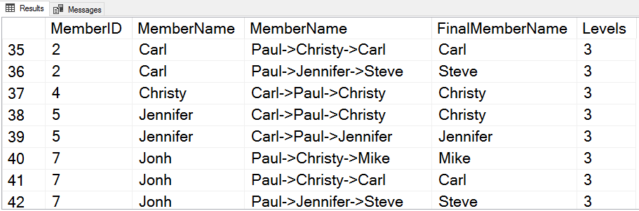
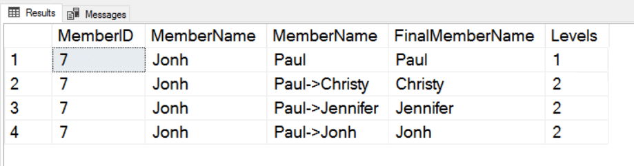
The image below gives an idea of the result. You have the information about the first member of the path, you have the entire path (not including the first member) created by the function STRING_AGG, you have the last name of the path created by the LAST_VALUE function, and you also have the number of levels in the path, created by the function COUNT
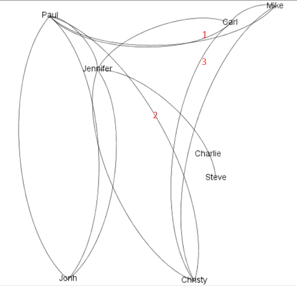
You may be wondering about how Carl connects to Carl. This image shows the path:
Performance
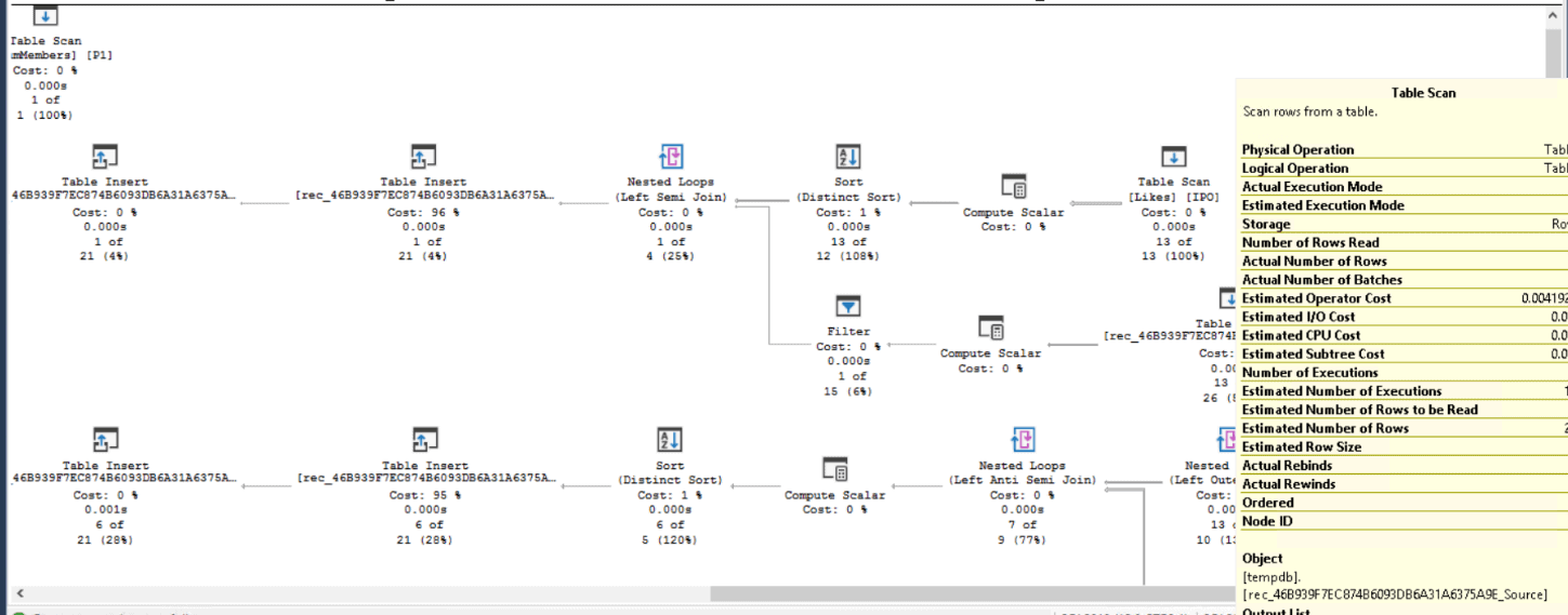
The execution plan is big. There is no doubt that you will need to take care when using it in large environments. The full execution plan doesn’t fit here, but you may notice by the piece below that the plan makes extensive use of tempdb.
You may notice the following details in the execution plan:
- It starts with the edge table
- It creates three temporary tables from the edge table. You will see many table operations in the plan, but checking the names, you will notice there are only three
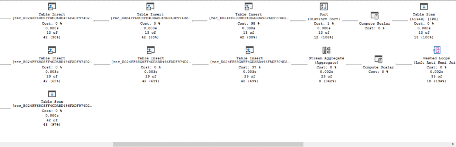
- It joins one of the temporary tables with the edge table, the nodes table and a second temporary table, aggregating the result and inserting in the temporary tables
- It has a
Sequenceoperator, which then is joined with the node table to get the results
Filtering
By adding one more predicate, you can view just the paths starting from one forum member:
|
1 2 3 4 5 6 7 8 9 10 11 12 13 |
SELECT P1.MemberID, P1.MemberName, STRING_AGG(P2.MemberName,'->') WITHIN GROUP (GRAPH PATH) AS [MemberName], LAST_VALUE(P2.MemberName) WITHIN GROUP (GRAPH PATH) AS FinalMemberName, COUNT(P2.MemberId) WITHIN GROUP (GRAPH PATH) AS Levels FROM ForumMembers P1, ForumMembers FOR PATH as P2, Likes FOR PATH as IPO WHERE MATCH(SHORTEST_PATH(P1(-(IPO)->P2)+)) AND p1.MemberID=7; |
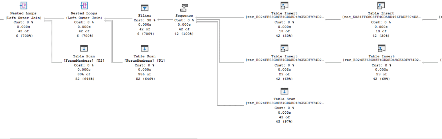
The execution plan changes. You may notice the following:
- The sequence is still the middle of the execution plan
- The plan starts by the node, not the edge
- After the sequence, the Query Optimizer is able to use an index for one of the nodes
- There is a fourth temporary table, called Source
- The number of paths before the sequence increases
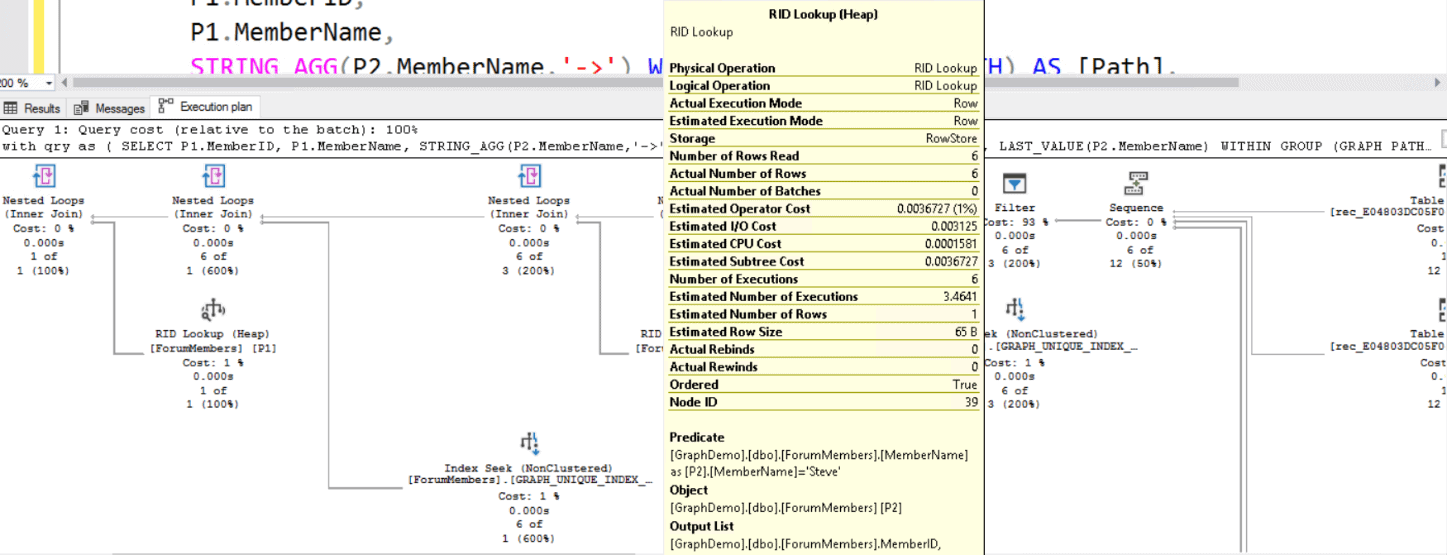
If you would like to see only the path between Jonh and Steve, you may be surprised that you have to separate the query into a CTE or subquery and filter the results. One reason is that a windowing function cannot be directly filtered. The MATCH statement doesn’t offer a solution either, you can’t filter by a P2 field, for example, because it’s marked as FOR PATH.
|
1 2 3 4 5 6 7 8 9 10 11 12 13 14 15 16 17 |
WITH qry AS ( SELECT P1.MemberID, P1.MemberName, STRING_AGG(P2.MemberName,'->') WITHIN GROUP (GRAPH PATH) AS [Path], LAST_VALUE(P2.MemberName) WITHIN GROUP (GRAPH PATH) AS FinalMemberName, COUNT(P2.MemberId) WITHIN GROUP (GRAPH PATH) AS Levels FROM ForumMembers P1, ForumMembers FOR PATH as P2, Likes FOR PATH as IPO WHERE MATCH(SHORTEST_PATH(P1(-(IPO)->P2)+)) and p1.MemberID=7) SELECT * FROM qry WHERE FinalMemberName='Steve'; |
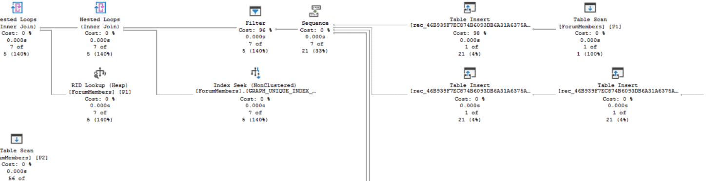
It’s not difficult to predict: The query plan is bad. You are calculating the path from Jonh to all other members and only after this does the filter kick in to get the path between Jonh and Steve. In the image below you may notice the filter for Steve only after the sequence, after calculating all the paths from Jonh
You may have already noticed the + symbol in the Match clause. It means you allow an unlimited number of hops. However, you can use a slightly different syntax to find all the forum members that are, for example, up to two hops away from others:
|
1 2 3 4 5 6 7 8 9 10 11 12 13 |
SELECT P1.MemberID, P1.MemberName, STRING_AGG(P2.MemberName,'->') WITHIN GROUP (GRAPH PATH) AS [MemberName], LAST_VALUE(P2.MemberName) WITHIN GROUP (GRAPH PATH) AS FinalMemberName, COUNT(P2.MemberId) WITHIN GROUP (GRAPH PATH) AS Levels FROM ForumMembers P1, ForumMembers FOR PATH as P2, Likes FOR PATH as IPO WHERE MATCH(SHORTEST_PATH(P1(-(IPO)->P2){1,2})); |
However, the start needs always to be 1. If you want to see the people that are an exact number of hops from other, once again you will need to filter the result of the query:
|
1 2 3 4 5 6 7 8 9 10 11 12 13 14 15 |
WITH qry as ( SELECT P1.MemberID, P1.MemberName, STRING_AGG(P2.MemberName,'->') WITHIN GROUP (GRAPH PATH) AS [path], LAST_VALUE(P2.MemberName) WITHIN GROUP (GRAPH PATH) AS FinalMemberName, COUNT(P2.MemberId) WITHIN GROUP (GRAPH PATH) AS Levels FROM ForumMembers P1, ForumMembers FOR PATH as P2, Likes FOR PATH as IPO WHERE MATCH(SHORTEST_PATH(P1(-(IPO)->P2){1,2})) ) SELECT * FROM qry WHERE levels=2; |
The shortest_path function is a great new feature for the SQL Server graph database, but being unable to filter the end node or the exact number of hops without performing the entire calculation and only then filter the result is still a problem for query performance.
Indexing
You can create indexes on the pseudo-columns of the edge and nodes. Considering the execution plans you saw, you can create the following clustered index for the edge:
|
1 |
CREATE CLUSTERED INDEX indLikes ON likes($from_id,$to_id); |
For the nodes, on the other hand, the index didn’t help so much. If you create a clustered index, it will result in a scan operation. If you create a non-clustered index, you would need to include all the columns involved in the operation. It may sound a bit strange, but one of the columns is the graph_id. There is no pseudo-column for the graph_id in the nodes table. There is one function to retrieve the graph_id, GRAPH_ID_FROM_NODE_ID, but you can’t use this function to create a computed column. This instruction bellow, for example, will fail:
|
1 2 3 |
ALTER TABLE forumMembers ADD graph_id AS (GRAPH_ID_FROM_NODE_ID($node_id)) PERSISTED; |
On the other hand, for the queries where you are filtering for the start member, a non-clustered index on the member id helps:
|
1 |
CREATE NONCLUSTERED INDEX indMembers ON ForumMembers(memberid); |
There is not much news about the more complex situations filtering by levels or end node: It’s an additional filter after all the calculations of shortest_path.
Conclusion
The function shortest_path is an excellent addition to the graph database features; however, the two limitations it has may create heavy queries in the environment:
- You can’t specify an end node.
- You can’t specify a start number of hops which would allow selecting an exact number of hops with same start and end.
This document contains proprietary information and is protected by copyright law.
Copyright © 2026 Red Gate Software Limited. All rights reserved


Load comments