Beginning with SQL Server 2012, you can now define columnstore indexes on your database tables. A columnstore index stores data in a column-wise (columnar) format, unlike the traditional B-tree structures used for clustered and nonclustered rowstore indexes, which store data row-wise (in rows). A columnstore index organizes the data in individual columns that are joined together to form the index. This structure can offer significant performance gains for queries that summarize large quantities of data, the sort typically used for business intelligence (BI) and data warehousing.

The Columnstore Structure

Columnstore indexes are based on xVelocity (formerly known as VertiPaq), an advanced storage and compression technology that originated with PowerPivot and Analysis Services but has been adapted to SQL Server 2012 databases.

At the heart of this model is the columnar structure that groups data by columns rather than rows. To better understand how this structure works, let’s look at a simple table (AutoType) that stores automobile-related data. The following T-SQL code shows the table definition:

Nothing elaborate here, just a few columns configured with basic types. But note that the AutoID column is configured as the primary key, which means that SQL Server will automatically create a clustered index based on that column. As is typical of a clustered index, the index’s leaf nodes store the data by rows, and each row includes all the data associated with that row. In addition, the data is spread across one or more data pages, as illustrated in Figure 1.

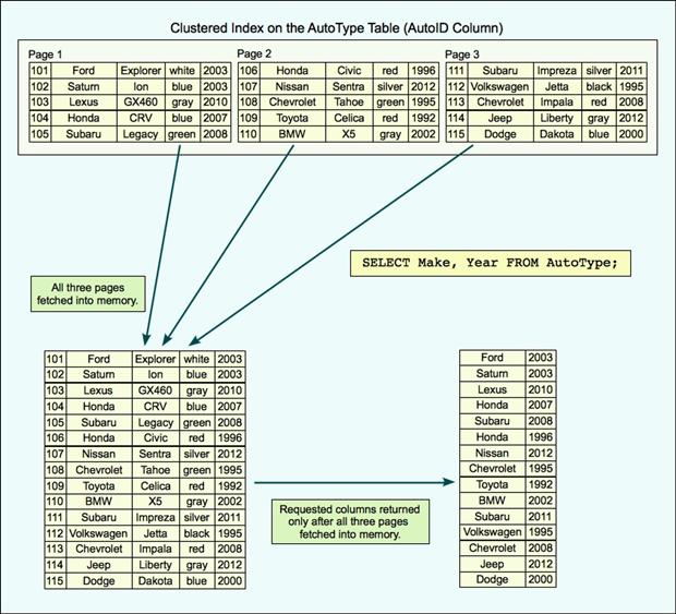
Figure 1: Retrieving data from a clustered index

In this case, the data is split across three pages, with each containing five rows. This, of course, is a highly unlikely scenario because each page would normally hold far more data, but for demonstration purposes, this setup should work fine. The important point to note is that each row is stored on a page in its entirety.

Now suppose we run the following query against the AutoType table:

When the database engine processes the query, it retrieves all three data pages into memory, fetching the entire table even though most of the columns aren’t needed. In other words, the system wastes valuable I/O and memory resources to retrieve unnecessary data.

Now let’s look at what happens when we create a columnstore index on the table. In this case, we’re including all columns in the index, to be consistent with our clustered index, though in actually we would probably include only some of the columns. Whatever columns we include, all of them are stored as columns within the index. Figure 2 illustrates what such an index might look like. As you can see, the data is no longer stored by row.

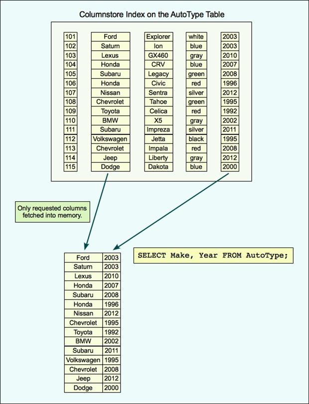
Figure 2: Retrieving data from a columnstore index

In the columnstore index shown in the figure, each column is its own segment. A segment can contain values from one column only, which allows each column’s data to be accessed independently. However, a column can span multiple segments, and each segment can be made up of multiple data pages. Data is transferred from the disk to memory by segment, not by page.

A segment is a highly compressed Large Object (LOB) that can contain up to one million rows. The data within each column’s segment matches row-by-row so that the rows can always be assembled correctly. For example, the second row in each segment in Figure 2 all point to the same car: the blue 2003 Saturn Ion with an ID of 102. The matched rows across all segments form a row group. We’ll look at row groups in more detail shortly, but first let’s return to our SELECT statement.

If we run the statement again, after creating our columnstore index, the query processor will use the columnstore index, rather than the clustered index. As a result, only the segments associated with the Make and ModelYear columns will be pulled into memory, thus limiting the resources necessary to process the query. This is especially important to disk I/O. Although we’ve seen giant leaps in processing and memory power, I/O remains a query’s weakest link, but the columnstore structure can help to reduce I/O significantly.

Of course, a column’s data won’t always fit into a single segment, given the one-million-row limitation. In such cases, multiple segments are created for each column and grouped into multiple row groups, one for each set of segments.

When a columnstore index is broken into multiple row groups, each row group contains a set of complete rows. For instance, Figure 3 shows our columnstore index now broken into three row groups. Each row group contains a segment for each column, and together those segments contain the complete set of rows.

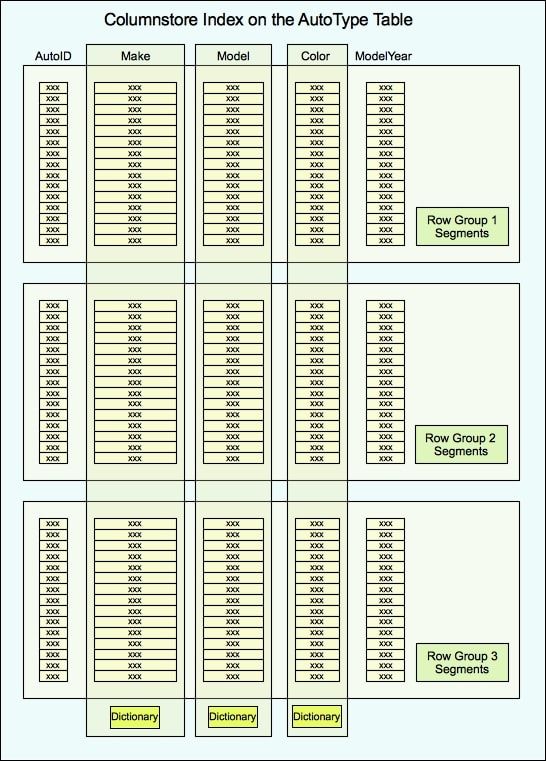
Figure 3: A columnstore index broken into three row groups

Notice that Figure 3 also shows several dictionaries, each associated with a specific column. A dictionary encodes the values in a column configured with a string data type or, in some cases, a non-string type if the column contains few distinct values. Although not all columns use dictionaries, all string columns do.

When a dictionary is used, it stores the column’s actual data values, and numerical reference values are inserted into the segments in place of those values. This can offer a great performance advantage for columns that contain many repeated values, but it can have a negative impact on columns with lots of unique values. Even so, a string column always uses a primary dictionary and might even use a secondary dictionary.

The Columnstore Index in Action

As noted above, one of the biggest advantages provided by a columnstore index is to reduce I/O, which can have a direct impact on query performance. Just to give you a taste of this, let’s look at a simple example. The following SELECT statement retrieves data from the FactResellerSales table in the AdventureWorksDW2012 sample database:

The table definition includes a composite primary key defined on the SalesOrderNumber and SalesOrderLineNumber columns, which form the basis of the table’s clustered index. As a result, when the query is executed, the query processor performs a clustered index scan. Figure 4 shows the query’s execution plan.

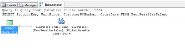
Figure 4: Execution plan showing a clustered index scan

Nothing too surprising here. Because the table contains only 60,855 rows, the query is processed almost instantaneously. Even so, it’s worth taking a quick look at the execution plan details, shown in Figure 5. Of particularly note is the estimated I/O cost of 2.19868. Notice that this represents a significant portion of the total operator costs of 2.26578. The remainder of the operator cost goes to the CPU, which comes in at only 0.0670975.

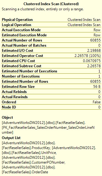
Figure 5: Viewing details about the clustered index scan

Now let’s create a columnstore index on our table. The following statement creates an index named csi_FactResellerSales on the ProductKey, UnitPrice, CustomerPONumber, and OrderDate columns:

Creating a columnstore index is as simple as creating any type of nonclustered index. (SQL Server doesn’t support clustered columnstore indexes.) Even so, there are plenty of dos and don’ts, so you might want to check out the topic “CREATE COLUMNSTORE INDEX (Transact-SQL)” in SQL Server Books Online or at MSDN before you create any of your own.

Once we create the columnstore index, we can rerun our query. The SELECT statement once again returns our rows instantaneously, this being such a small data set, but produces a different execution plan, as shown in Figure 6.

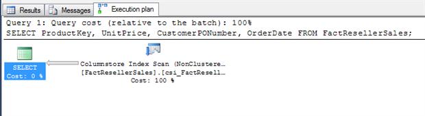
Figure 6: Execution plan showing a columnstore index scan

As you can see, this time the query processor performs a columnstore index scan, rather than a clustered index scan. A quick review of the execution plan details, shown in Figure 7, reveals a very different I/O picture.

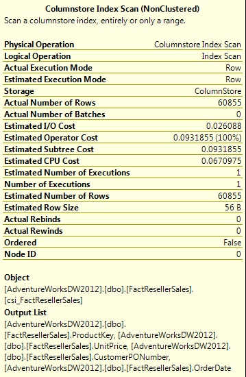
Figure 7: Viewing details about the columnstore index scan

Notice first of all that out CPU costs are the same as they were for the clustered index: 0.0670975. However, our operator cost this time around is only 0.0931855, compared to 2.26578 for the clustered index. That’s because our I/O cost is now only 0.026088, rather than the 2.19868 returned by the query using the clustered index.

This example is undoubtedly a very simple and lightweight one, but it does demonstrate how the columnar nature of columnstore indexes can reduce I/O costs in your queries. However, the indexes’ columnar structure is not the only aspect of the columnstore index that can result in performance gains. Compression also plays an integral role.

Columnstore Compression

Compression certainly isn’t new to SQL Server. However, because data in a columnstore index is grouped by columns, rather than by rows, data can be compressed more efficiently than with rowstore indexes. Data read from a single column is more homogenous than data read from rows, and the more similar the data, the easier it is to compress. Add to that equation a low number of distinct values and the use of dictionaries, and the advantages only grow.

The xVelocity technology also brings with it sophisticated compression algorithms that can take full advantage of the indexes’ columnar nature. And the more effectively you can compress your data, the more data you can fit on a single page and the more data you can pull into memory, both of which lead to a lower I/O costs. If you consider the nature of BI workloads, which often involve aggregating large data sets, you can see the clear advantage of the columnstore structure. The need for the increased CPU power that such aggregation requires can be offset by the I/O savings, helping to improve the performance of those gargantuan queries that were bogging down your systems before the columnstore index came along.

Batch Mode Processing

Working with highly compressed columnar indexes is certainly a great start when taking on those BI workloads. But SQL Server 2012 adds another element to the mix to improve performance even more: batch mode processing. Analytical BI queries must often scan extremely large sets of data and perform numerous complex operations, even to produce a small result set. Batch mode processing can operate on many rows at a time-a batch-rather than one row at a time, as is typical with row-mode processing, the type used for most online transactional processing (OLTP) operations.

In SQL Server 2012, when the query processor executes a query, it can use batch mode, row mode, or both. To use both, the query optimizer can create plans that include sub-trees in batch mode even if the main tree is in row mode. However, the goal is to try to get your queries to run in batch mode from beginning to end, and if that’s not possible, to get as much of the query as you can to use batch mode. Even in mix mode, you’re likely to see performance gains.

But not all operations will run in batch mode. Some of these limitations are inherent in SQL Server 2012, and there’s little you can do to work around them. In other cases, you might be able to tweak your queries to maximize batch mode processing. For information on several steps you can take to get your queries to use batch mode, refer to the TechNet Wiki article “SQL Server Columnstore Performance Tuning.” Keep in mind, however, the advantages of batch processing can be realized only if you’re joining, filtering, or aggregating large data sets. Without these elements, batch processing is not possible.

The SQL Server 2012 Columnstore Index

Columnstore indexes, along with batch mode processing, have been optimized with data warehouses in mind, specifically when the indexes are created on fact tables. You’ll see the best performance on large fact tables with small-to-medium dimension tables configured in a star schema, better still if the included columns contain many repeated values. Yet even if you meet these criteria, the performance gains might be minimal if you’re returning large, non-aggregated result sets, joining tables too large to fit into memory, returning or joining too many columns, or running queries not using batch processing mode.

A columnstore index also has a number of limitations and restrictions (too many to list here), such as which data types can be indexed, the number of columns that can be included, the type of objects that support columnstore indexing, and numerous other considerations. For more details about what you can and cannot do with column store indexes, see the topic “Columnstore Indexes” in SQL Server Books Online or at MSDN. The topic also includes details about how to update data in a columnstore index. Essentially, you can’t do it, but you can take steps such as dropping the index or partitioning the table.

Despite the limitations of the columnstore index, they can provide performance improvements that far exceed what you can get with the rowstore structures of clustered and nonclustered indexes. When used under the right circumstances, columnstore indexes can significantly reduce disk I/O and well as utilize memory more efficiently. These indexes are made for the type of analytical processing your BI workloads often require, an important consideration in this age of ever increasing data.