The R platform and programming language supports a vast array of data science techniq. With decades of history and over 7,000 packages available on CRAN it can be overwhelming to determine where to start. The R-Basics and Visualizing Data with R articles provide initial direction, but don’t go into much detail about how to manipulate datasets within R. 

Fortunately, database professionals can be productive quickly in this realm by leveraging their well-honed SQL skills.  As you might expect, R supports the use of SQL to retrieve data from centrally located relational databases. However, several packages in R allow you to go beyond this realm and create and query ad-hoc datasets on the fly in the midst of processing and analyzing data, regardless of the data’s original source or final destination. In this article, we will look at several different approaches that involve manipulating data with SQL using various R packages.

There is a great deal of excitement regarding Microsoft’s acquisition of Revolution Analytics that subsequently lead to R being integrated into SQLServer 2016.  SQLServer 2016 is available as a preview, but is still subject to changes before its official release. Simple-talk is filled with excellent articles that focus specifically on SQLServer. Once the details of the release are finalized, you can expect more upcoming articles that uniquely address R as implemented within SQLServer. But since the final version of SQLServer is not yet available at this time, and Simple-Talk has already covered SQL Server Access from R, this article will demonstrate open source R in RStudio using SQL with other relational databases.

Part of the appeal of SQL is its availability in so many different products.  Most technical professionals find themselves having to support and interact with a range of technologies from both open source and commercial vendors. Despite vendor-specific features and extensions, SQL is relatively standard across implementations so its use as presented here will be familiar even to those who currently work exclusively with SQLServer. This article will include references to two databases, SQLite, a small freely available (public domain) database that many people use without even knowing it and Oracle, a large commercial offering and competitor to SQLServer. The use of RODBC to access SQL Server has already been covered in the Simple-Talk article ‘Making Data Analytics Simpler: SQL Server and R’

The RSQLite package

SQLite is the most widely deployed database in the world. It is included on Android, iPhone and IOS devices and in Firefox, Chrome and Safari web browsers. Apple and Microsoft include it in their OSX and Windows 10 operating systems respectively and there are many other products that include SQLite. It is extremely easy to use, and can be of great value to developers who need a database available but want to avoid the overhead often associated with installing and configuring an external database. In this demonstration, we will download and install the RSQLite package which will integrate SQLite into R running in RStudio. 

This example will show how data sets can seamlessly be written into a SQLite database for subsequent analysis using familiar SQL statements (the data in question pertains to automobile performance and fuel efficiency). The dataset is included with R during its initial installation. Since the included data is readily available within R, it is not necessary to import the data from a spreadsheet or other external source. Such datasets are used in examples in R documentation, so they are available within R during its initial installation, or are added along with code when new packages are installed.

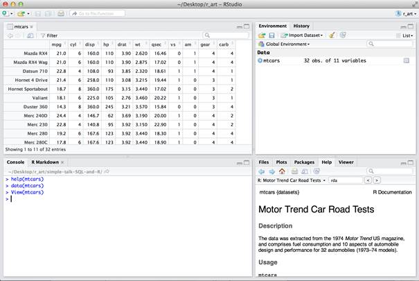
The “mtcars” dataset is included by default in R. It consists of data from the 1974 Motor Trend US magazine (hence the “mt” in the dataset name). The dataset describes fuel consumption and various aspects of automobile design and performance for 32 automobiles. The help function will display a document that contains in-depth description of the structure and contents of this dataset.

In order to access this dataset, it must first be loaded. This “attaches” the dataset to the user’s current R session.  

The dataset is represented in an object called a data frame comprised of rows and columns. The data frame is small enough to be easily perused in a spreadsheet-like display using the View command. 

If you want to remove the dataset from your session at a later point to free up resources without exiting R, you can run the rm function. When you run this command, you will notice the mtcars variable listed in the Environment pane will disappear.

Within RStudio, the SQLite package must be installed unless it had been previously installed. The library function then can be called to load the package into the current working environment.

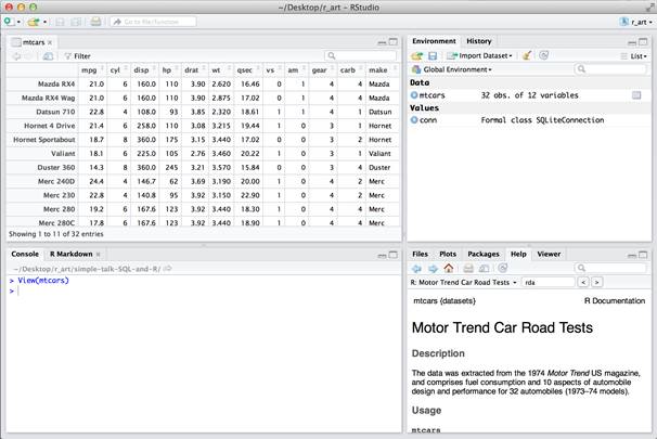
Next we will create a new, empty SQLite database where we can store the cars data. SQLite has a rather simple data storage mechanism, all data for a database is installed within a single file.  The name of this file must be specified when the database is created, and a connection to this database is returned and used in subsequent commands to access and manipulate the data and data structures within the database.

This command creates a file named “mycars.db” in the current working directory. If you aren’t sure where this is, run getwd() to print out your working directory and setwd(“some-directory”) to navigate to a different directory. To actually create a table, we will read data from the mtcars dataset and write it to the new database.

With the data loaded, and an active database connection to the SQLite database, we can write the data by specifying the connection, the name of the table, and the name of the data frame that contains the data to be persisted.

This simple statement created a table in the database with data types analogous to the R data frame columns. The names of the table columns were based on the names of the columns in the data frame. No complicated CREATE TABLE statement was required with explicit definitions of column names, data types, precision, storage configuration or other options. This level of detail is unnecessary when the focus is on performing an ad-hoc exploratory data analysis within R rather than defining a schema in a centralized database that is intended for long-term use.  However, it is possible to run CREATE TABLE statements if you like to using standard SQL DDL.

SQLite, like other relational database stores metadata describing the objects it contains. The tables in the database can be listed by a single function call. 

Likewise, the field names for a given table can be listed referencing the connection and the table name.

With a connection available, a database created and a table populated with data, queries can now be executed using the dbGetQuery function.

Standard SQL syntax is available, though as in other contexts where SQL is embedded in strings, you need to consider your usage of quotes. Often it is simplest to surround your queries with double quotes so that strings in a SQL statement can be surrounded in single quotes.

As you might expect, modifying tables using SQL is also possible using RSQLite. But there is a shortcut if the case where a data frame is modified in the context of R with the intention of overwriting a table previously created. The following example extracts the “make” of the car from the row name where the make and model are concatenated. 

This statement says in essence, “create a new column for the data frame named “make” and populate each row’s make value by taking the row name, finding the substring that starts with the first space and ends at the end of the string, and removing that substring.” What remains is the first word in the string. The resulting data frame can be viewed to reveal the new make column appended as the last column.

The new column can now be used in queries like any of the other columns.

The RSQLite package makes it easy to take data from files, spreadsheets, or other sources and quickly integrate it into a SQL accessible database. It allows you to do a great deal of data processing without requiring the additional time, resources and effort needed to set up and maintain an external database. As convenient as this is, another package called sqldf simplifies this type of processing even further. It allows you to use SQL on data frames without giving any thought to setting up a database at all.

The sqldf package

There is tremendous value in consistently using SQL (or SQL-like) languages to explore and process data.  Data Science professionals are frequently faced with the challenge of integrating data from disparate data sources. Many of these are relational databases, and so require SQL to retrieve data. In addition, NoSQL data sources often support high level, declarative, SQL-like languages. For example, Hadoop users can use Hive and Pig. Cassandra provides access to data stored in column families (analogous to relational tables) using Cassandra Query Language (CQL). In many cases data in arbitrary text files is structured enough to be easily imported into a database, and a variety of utilities are commonly used to make semi-structured data SQL accessible. Thinking about data in relational terms lends itself towards Tidy data formatting that has value even outside of the relational realm.

The sqldf package allows you to access data frames using SQL. Regardless of where data originates, it can be queried as long as it is contained within a data frame. This means that data can  be read in from a variety of data sources (delimited files, a web pages, web APIs, a relational databases, NoSQL datasoures, etc) and subsequently queried and manipulated as if it were all in a single relational database. To see how straightforward it is, open a new R Session, install the package, load it and the mtcars data.

SQLDF allows you to query the data frame as if it were a table and it is often as simple as passing the query as a string to the sqldf function.

If you are following along and executed this statement in RStudio, the number of rows is correct, but the row names containing the name of each car are missing.

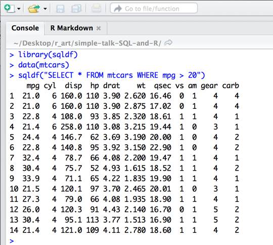
The reason is that row names are not standard columns and are ignored by default by sqldf. To include these rows in the output, specify row.names=TRUE when making the call.

Within R, there are many ways to create new data frames. The base language contains support, and packages like dplyr and reshape are in common use. With sqldf, you can bypass the use of all of this. In fact, the sqldf call itself returns a dataframe. With this in mind, you can do sequences of calls to sqldf to incrementally process or summarize a data set.

The df object now contains a dataframe with the results of the query. If you are going to process a data frame in this way, you are better off making the row names an ordinary column value.

The new column is now available in the dataframe. And any result of a query, even if it varies widely from the original is simply returned as a new data frame.

The judicious use of aliases to have meaningful column names in each new dataset will make it easier to do subsequent processing. Limiting yourself to alphanumeric characters for column names is recommended.

The SQL used with sqldf will mirror that used by RSQLite since behind the scenes, data is being written to SQLite tables for querying.  

The mtcars data set internally available in R is convenient for examples. Although it is great for quickly demonstrating or learning functionality, it is not sufficient for real world applications where data must be retrieved from an external source.

File Imports

Before looking at making direct connections to a database, it is important to recognize how simple and straightforward it is to read a delimited file into RStudio. This might be somewhat offensive to software developers who are accustomed to creating applications that connect directly to databases using ODBC or JDBC.  But R Users frequently need to integrate data from several different data sources. Rather than expend time and energy configuring specific packages and loading drivers, it be worth considering exporting data from a query to a data file and reading the file into RStudio. This practice can also circumvent the need to run resource intensive SQL statements multiple times on a database.

Exporting data as CSV is a well supported option in many relational database systems. SQLServer’s Management Studio has a “Results To Text” dialog where “Comma delimited” can be specified as an output format. MySQL has a non-standard SQL SELECT clause to specify an OUTFILE clause. Many SQL Clients include an option to export data in this way. CSVs exported from databases can be quickly validated using any spreadsheet program.

R itself can import data from a wide variety of file formats. This flexibility results in additional complexity, specifically a long list of functions, many of which have a large number of parameters that can be set to alter their behavior. RStudio masks this complexity and provides a simple dialog for importing files.  If you don’t have a CSV file  handy, you can start by creating one using R based on the mtcars dataset we saw earlier.

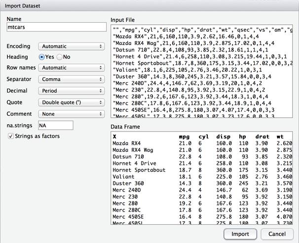
Import this by selecting the “Import Dataset” option in the Environment pane and choosing “From Text File”.

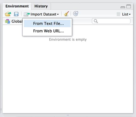
A dialog is opened that provides a preview of how the data will be imported based on the options selected. In most cases, uncheck stringsAsFactors and the defaults selected will suffice. 

As the data is imported, the actual R commands required to read in and view the data are displayed inline in the console. The data is first read into R.

The View function is then called on the new data frame to display its contents.

If you wish, the read.csv command can be set aside and used in a script making it unnecessary to import data interactively using the dialog in the future.

Because of data can often be conveniently be exported to simple text files, they are frequently the simplest way to get data into RStudio. This is not always the case of course. At times, when working with a relational database the amount of data being processed is prohibitive, or the number of data frames to be created makes it unwieldy to manually export and import multiple data files. Under these circumstances, a direct connection to the database is the best option. There are a number of database specific packages that support direct connections. Most of these packages are based on the RJDBC package, and the RJDBC package can be used independently to access a large variety of databases.

The RJava and RJDBC Package

JDBC is the Java analog to the ODBC standard that was original developed by Microsoft. A JDBC driver is software that enables a Java application to interact with a specific database. The RJDBC package therefore relies upon the RJava package and consequently on an underlying Java installation on an R User’s machine. At times, the behavior of the Java Virtual Machine must be addressed to prevent problems. For instance, if you encounter OutOfMemoryExceptions, the solution is to increase the amount of memory available to the JVM.

Suffice it to say that there are a wide range of configuration possibilities that can result in problems due to the myriad of possible permutations of versions of R, Java, RJDBC, particular JDBC drivers and a specific database. These are virtually unheard of when using a vendor-specific version of R included with a particular database (as is the case with OracleR and Microsoft SQLServer 2016), but they are not uncommon when using RJDBC to make database connections. Again, the previous section describes exporting/importing csvs as a viable workaround worth considering if you encounter these sorts of issues. RJDBC problems are not unsolvable, just time-consuming. Projects that involve a one-time data dump don’t merit the attention required to fix them.

Install and load the RJDBC library.

This example uses the free Oracle XE database and a pre-installed demo account called HR. Note that in this case, the database installation itself is on a local workstation, but completely external to R. Before running the R code, you must ensure that the HR user account is available. From an operating system prompt, connect as a user with DBA privileges. 

Within SQL*Plus, unlock the HR account and set the password to match the username.

RJDBC requires the use of a JDBC driver, in this case an Oracle JDBC driver that was installed as part of Oracle’s Instant Client is used. The code below includes a Java CLASSPATH that is specific to my personal machine that must be modified to match your setup. It loads the JDBC driver which is then used to make a database connection.

A connection is established using the loaded driver, a JDBC URL, and the user and password associated with the HR account.

The connection is then passed in each call along with the query.

This query displays all of the tables available within the HR user’s schema.

Conclusion

There is plenty that is novel and perhaps foreign to a new R user. But there is no reason to abandon your hard-earned SQL skills. The RSQLite, SQLDF and RJDBC packages allow you to leverage your SQL skills whether accessing external data or simply cleaning, filtering and modifying data already loaded. When SQLServer is released, the ease of integration of using the version R included will likely enhance this synergy. R’s flexibility in accessing other data sources will provide new opportunities to create data-centric products and services that are far beyond what was traditionally possible using SQL alone.