
Since SQL Server 2005, there has been a database option which can be SET at database level called DATE_CORRELATION_OPTIMIZATION: This feature is OFF by default. Personally, I have never seen anyone use this feature, but I believe that this is only because there is so little material around that refers to, or explains, this feature.
It is very important that the developer or DBA knows the type of application and database query that would benefit of this feature, since it can produce striking increases in performance; but, at this point, you are probably wondering, ‘what does this feature actually do?’
Tying Dates together
When enabled, the DATE_CORRELATION_OPTIMIZATION allows the Query Optimizer to improve the performance of certain queries by gathering some statistical information about the DATETIME columns of two tables which are linked by one-column foreign key. This collected data is generally known as correlation statistics (not to be confused with Query Optimization Statistics), because they help the Query Optimizer to identify a correlation between two DATETIME columns. With this information, the Query Optimizer can make the best decision to obtain a better execution plan, and which data can be filtered to avoid unnecessary page reads.
Let’s try an example: we have one table with some Orders (Pedidos) and a column called OrderDate(Data_Pedido), and another table called OrderItems(Items) and a column called DeliveryDate (Data_Entrega) where the delivery date is not equal to the order date but where the delivery date is within a range of dates after an order. In other words, where the two dates correlate, but are not equal. As an example of this, Imagine that I’ve made a purchase at submarino.com.br, buying a lot of different products, from books to a plush toys. Perhaps I ought to explain that my wife likes penguins, so I buy one. Anyway, despite the fact that I only made one order, I received each product on different days, because each product came from different places.
In this example, we have a table called orders with the date of the order, and a table called OrderItems with the delivery date of each product. We can be fairly confident in saying that the date of order is always very close to the delivery date of each item. That represents a clear correlation between the OrderDate and the DeliveryDate.
I hope that this explains what is meant by a correlation between the two DATETIME columns. So let’s get back to the optimization.
Suppose you have a query which has a join between the Order and OrderItems columns, and you are doing a filter in one of DATETIME column, the SQL Server can modify your query to make that better without you seeing any change; All internally and automatically. How? Let’s go start with an example.
First of all we’ll create one metadata to allow us see tables close to the example I’ve described.
The names of the tables are in Portuguese, but I’m sure this will not be a problem to you.
|
1 2 3 4 5 6 7 8 9 10 11 12 13 14 15 16 17 18 19 20 21 22 23 24 25 26 27 28 29 30 31 32 33 34 35 36 37 38 39 40 41 42 43 44 45 46 47 48 49 |
IF OBJECT_ID('Pedidos') IS NOT NULL BEGIN DROP TABLE Items DROP TABLE Pedidos END GO CREATE TABLE Pedidos(ID_Pedido Integer Identity(1,1), Data_Pedido DateTime NOT NULL,--The columns cannot accept null values Valor Numeric(18,2), CONSTRAINT xpk_Pedidos PRIMARY KEY (ID_Pedido)) GO CREATE TABLE Items(ID_Pedido Integer, ID_Produto Integer, Data_Entrega DateTime NOT NULL,--The columns cannot accept null values Quantidade Integer, CONSTRAINT xpk_Items PRIMARY KEY NONCLUSTERED(ID_Pedido, ID_Produto)) GO -- At least one of the DATETIME columns, must belong to a cluster index CREATE CLUSTERED INDEX ix_Data_Entrega ON Items(Data_Entrega) GO -- There must to be a foreign key relationship between the tables that contain correlation date ALTER TABLE Items ADD CONSTRAINT fk_Items_Pedidos FOREIGN KEY(ID_Pedido) REFERENCES Pedidos(ID_Pedido) GO DECLARE @i Integer SET @i = 0 WHILE @i < 10000 BEGIN INSERT INTO Pedidos(Data_Pedido, Valor) VALUES(GetDate() - ABS(CheckSum(NEWID()) / 10000000), ABS(CheckSum(NEWID()) / 1000000)) SET @i = @i + 1 END GO INSERT INTO Items(ID_Pedido, ID_Produto, Data_Entrega, Quantidade) SELECT ID_Pedido, ABS(CheckSum(NEWID()) / 10000000), Data_Pedido + ABS(CheckSum(NEWID()) / 100000000), ABS(CheckSum(NEWID()) / 10000000) FROM Pedidos GO INSERT INTO Items(ID_Pedido, ID_Produto, Data_Entrega, Quantidade) SELECT ID_Pedido, ABS(CheckSum(NEWID()) / 10000), Data_Pedido + ABS(CheckSum(NEWID()) / 100000000), ABS(CheckSum(NEWID()) / 10000000) FROM Pedidos GO |
After the tables are created, we’ll have one structure close to what has been presented above, let’s go see one sample of the data.
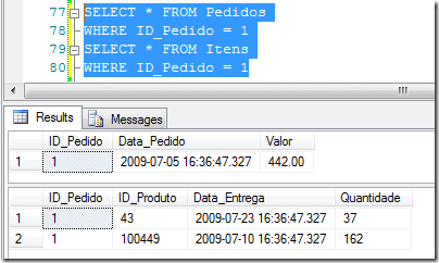
Now, suppose one developer builds the following query.
|
1 2 3 4 5 |
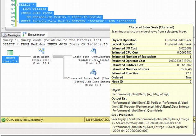
SELECT * FROM Pedidos INNER JOIN Items ON Pedidos.ID_Pedido = Items.ID_Pedido WHERE Pedidos.Data_Pedido BETWEEN '20090301' AND '20090305' |
Translating, I want all data from Orders and Items sold between 2009/03/01 and 2009/03/05. To this query the Query Optimizer created the follow execution plan:
SELECT * FROM Pedidos INNER JOIN Items ON Pedidos.ID_Pedido = Items.ID_Pedido WHERE Pedidos.Data_Pedido BETWEEN ‘20090301’ AND ‘20090305’
|–Hash Match(Inner Join, HASH:([Performance].[dbo].[Pedidos].[ID_Pedido])=([Performance].[dbo].[Items].[ID_Pedido]))
|–Clustered Index Scan(OBJECT:([Performance].[dbo].[Pedidos].[xpk_Pedidos]), WHERE:([Performance].[dbo].[Pedidos].[Data_Pedido]>=’2009-03-01′ AND [Performance].[dbo].[Pedidos].[Data_Pedido]<=’2009-03-05′))
|–Clustered Index Scan(OBJECT:([Performance].[dbo].[Items].[ix_Data_Entrega]))
In the text execution plan, we can easily see that the filter specified in the WHERE clause, was applied where the data was reading from index xpk_Pedidos, and the column which was received the filter was just the Data_Pedido specified in the WHERE clause.
The first thing we could do to optimize this query, is to create one index based on Data_Pedido column. You may be thinking that this would be the first thing that anyone would do with the query. Ok, you are right; but we will just create this index and continue with the optimization.
|
1 |
CREATE INDEX ix_teste ON Pedidos(Data_Pedido) INCLUDE(Valor) |
After create the index we have the follow plan:
SELECT * FROM Pedidos INNER JOIN Items ON Pedidos.ID_Pedido = Items.ID_Pedido WHERE Pedidos.Data_Pedido BETWEEN ‘20090301’ AND ‘20090305’
|–Hash Match(Inner Join, HASH:([Performance].[dbo].[Pedidos].[ID_Pedido])=([Performance].[dbo].[Items].[ID_Pedido]))
|–Index Seek(OBJECT:([dbo].[Pedidos].[ix_teste]), SEEK:([dbo].[Pedidos].[Data_Pedido] >= ‘2009-03-01’ AND [dbo].[Pedidos].[Data_Pedido] <= ‘2009-03-05’) ORDERED FORWARD)
|–Clustered Index Scan(OBJECT:([Performance].[dbo].[Items].[ix_Data_Entrega]))
Now the query is a little better, instead of making a Clustered Index Scan to read the data from Pedidos table, the SQL makes an Index Seek based on the index which we just created. Now, what else we could do to improve this further? It is time to see the Correlation_Optimization work.
As we can see, there is a point of bottleneck in the execution plan to read the data from the table Items: According to the execution plan, this read represents 49% of the entire cost, and the execution plan was using the clustered Index Scan operator to read the data from the table. If we could do something to use the Index Seek operator, then maybe the query could be improved. Is there something that we can do to the Query Optimizer use the Index Seek operator?
Knowing the database, the metadata and the business rules, we could modify the query to use one filter in the Items table. But, to do that, we need to be sure about this, because this change can’t modify the result of the query. One way to do this would be like:
- Based on the Orders between 2009/03/01 and 2009/03/05, look which are the min and the max delivery date from the Orders Items.
- With that information, put one new filter on the query to column Items.Data_Entrega.
After that, we have the following query:
|
1 2 3 4 5 6 |
SELECT * FROM Pedidos INNER JOIN Items ON Pedidos.ID_Pedido = Items.ID_Pedido WHERE Pedidos.Data_Pedido BETWEEN '20090301' AND '20090305' AND Items.Data_Entrega BETWEEN '20090301' AND '20090325 23:59:59.000' |
This way we could force a filter on the Items table as in the plan:
But, I now have a question. How to do to know the values specified on Item 1 and 2 above mentioned? Is there a way to know these values without searching the tables? The problem is that these values are not fixed values, but are variables.
What about letting the SQL Server Query Optimizer figure out that for you? All you need to do is to enable the DATE_CORRELATION_OPTIMIZATION, then the SQL Server Query Optimizer will identify that for you, and will apply the filter on the Data_Entrega column itself. Wow! pretty smart isn’t it? let me see if that is really true….
|
1 |
ALTER DATABASE <YOURDATABASE> SET DATE_CORRELATION_OPTIMIZATION ON; |
Let’s now run the query without the Data_Entrega filter again.
SELECT * FROM Pedidos INNER JOIN Items ON Pedidos.ID_Pedido = Items.ID_Pedido WHERE Pedidos.Data_Pedido BETWEEN ‘20090301’ AND ‘20090305’
|–Hash Match(Inner Join, HASH:([dbo].[Pedidos].[ID_Pedido])=([dbo].[Items].[ID_Pedido]))
|–Index Seek(OBJECT:([dbo].[Pedidos].[ix_teste]), SEEK:([dbo].[Pedidos].[Data_Pedido] >= ‘2009-03-01’ AND [dbo].[Pedidos].[Data_Pedido] <= ‘2009-03-05’) ORDERED FORWARD)
|–Clustered Index Seek(OBJECT:([dbo].[Items].[ix_Data_Entrega]), SEEK:([dbo].[Items].[Data_Entrega] >= ‘2009-02-28’ AND [dbo].[Items].[Data_Entrega] < ‘2009-04-29’) ORDERED FORWARD)
Look; this time, even when we have not specified the Data_Entrega filter, the Query Optimizer builds this for me.
Summary
The DATE_CORRELATION_OPTIMIZATION is a feature that is very good as a way of improving the performance of queries that use joins based on DATETIME values that are related but not necessarily equal, but it is almost never used outside specialized data-warehousing applications and BI. This may be because there needs to be a good analysis, and prior thought, about when and where this can be used.
All the following conditions must be met to this feature work:
- The database SET options must be set in the following way. All the following database options, ANSI_NULLS, ANSI_PADDING, ANSI_WARNINGS, ARITHABORT, CONCAT_NULL_YIELDS_NULL, and QUOTED IDENTIFIER must be SET to ON. NUMERIC_ROUNDABORT must be SET to OFF.
- There must be a single-column foreign key relationship between the tables.
- The tables must both have DATETIME columns that are defined NOT NULL.
- At least one of the DATETIME columns must be the key column of a clustered index (if the index key is composite, it must be the first key), or it must be the partitioning column, if it is a partitioned table.
- Both tables must be owned by the same user.
If you can meet these conditions and you are dealing with temporal data, then you could be in for a pleasant surprise
Load comments