
Gap-filling a time series – taking a sparse record of values-at-some-dates and producing a dense record of values-at-every-date-in-the-range, with missing values carried forward from the prior known value (LOCF imputation) – is a common data-prep task in financial reporting, inventory management, and time-series analysis.
This article presents a specific gap-filling challenge (filling a balance table with workday-level rows, carrying the last-known balance forward) and walks through three T-SQL solutions with measured performance: (1) TOP-based lookup using APPLY, which works on any version but has scan-heavy execution on large data; (2) IGNORE NULLS in SQL Server 2022+ combined with FIRST_VALUE, which is the cleanest modern solution; (3) range matching between the sparse values table and a workdays table using gaps-and-islands techniques, which is the most complex to write but best-performing at scale. Each solution is shown complete with performance numbers across several dataset sizes.
A student of mine sent me a T-SQL challenge involving gap-filling of missing dates and balances. I found the challenge interesting and common enough and figured that my readers would probably find it interesting to work on as well.
I’ll present the challenge and three possible solutions, as well as the results of a performance test. AS always, I urge you to try and come up with your own solutions before looking at mine.
If you would like to download the code including the solutions, you can find it in a .zip file here.
The Challenge
The challenge involves two tables called Workdays and Balances. The Workdays table holds the dates of all workdays going back a few years. The Balances table holds account IDs, dates of workdays when the account balance changed, and the balance on the current date. There’s a foreign key on the date column in the Balances table referencing the date column in the Workdays table.
Use the following code to create the Workdays and Balances tables:
|
1 2 3 4 5 6 7 8 9 10 11 12 13 14 15 16 17 18 19 20 21 |
SET NOCOUNT ON; USE tempdb; DROP TABLE IF EXISTS dbo.Balances, dbo.Workdays; GO CREATE TABLE dbo.Workdays ( dt DATE NOT NULL, CONSTRAINT PK_Workdays PRIMARY KEY(dt) ); CREATE TABLE dbo.Balances ( accountid INT NOT NULL, dt DATE NOT NULL CONSTRAINT FK_Balances_Workdays REFERENCES dbo.Workdays, balance NUMERIC(12, 2) NOT NULL, CONSTRAINT PK_Balances PRIMARY KEY(accountid, dt) ); |
Note that the definition of the primary key constraint on Workdays results in a clustered index with dt as the key. Similarly, the definition of the primary key constraint on Balances results in a clustered index with (accountid, dt) as the key.
To generate the sample data for this challenge, you will need a helper function that returns a sequence of integers in a desired range. You can use the GetNums function for this purpose, which you create using the following code:
|
1 2 3 4 5 6 7 8 9 10 11 12 13 14 15 16 17 18 19 20 21 |
CREATE OR ALTER FUNCTION dbo.GetNums (@low AS BIGINT = 1, @high AS BIGINT) RETURNS TABLE AS RETURN WITH L0 AS ( SELECT 1 AS c FROM (VALUES(1),(1),(1),(1),(1),(1),(1),(1), (1),(1),(1),(1),(1),(1),(1),(1)) AS D(c) ), L1 AS ( SELECT 1 AS c FROM L0 AS A CROSS JOIN L0 AS B ), L2 AS ( SELECT 1 AS c FROM L1 AS A CROSS JOIN L1 AS B ), L3 AS ( SELECT 1 AS c FROM L2 AS A CROSS JOIN L2 AS B ), Nums AS ( SELECT ROW_NUMBER() OVER(ORDER BY (SELECT NULL)) AS rownum FROM L3 ) SELECT TOP(@high - @low + 1) rownum AS rn, @high + 1 - rownum AS op, @low - 1 + rownum AS n FROM Nums ORDER BY rownum; |
Alternatively, if you’re using SQL Server 2022 or Azure SQL Database, you can use the built-in GENERATE_SERIES function instead. In my examples I’ll use the GetNums function.
Use the following code to populate the Workdays table with dates in 2013 through 2022 excluding weekends as sample data:
|
1 2 3 4 5 6 7 8 |
DECLARE @start AS DATE = '20130101', @end AS DATE = '20221231'; INSERT INTO dbo.Workdays(dt) SELECT A.dt FROM dbo.GetNums(0, DATEDIFF(day, @start, @end)) AS N CROSS APPLY (VALUES(DATEADD(day, N.n, @start))) AS A(dt) -- exclude Saturday and Sunday WHERE DATEDIFF(day, '19000107', dt) % 7 + 1 NOT IN (1, 7); |
Normally, dates of holidays would also be excluded from the table, but for our testing purposes we can keep things simple and just exclude weekends.
As for the Balances table; to check the logical correctness of your solutions, you can use the following code, which populates the table with a small set of sample data:
|
1 2 3 4 5 6 7 8 9 10 11 12 13 14 15 16 17 18 19 20 |
TRUNCATE TABLE dbo.Balances; INSERT INTO dbo.Balances(accountid, dt, balance) VALUES(1, '20220103', 8000.00), (1, '20220322', 10000.00), (1, '20220607', 15000.00), (1, '20221115', 7000.00), (1, '20221230', 4000.00), (2, '20220118', 12000.00), (2, '20220218', 14000.00), (2, '20220318', 16000.00), (2, '20220418', 18500.00), (2, '20220518', 20400.00), (2, '20220620', 19000.00), (2, '20220718', 21000.00), (2, '20220818', 23200.00), (2, '20220919', 25500.00), (2, '20221018', 23400.00), (2, '20221118', 25900.00), (2, '20221219', 28000.00); |
The task involves developing a stored procedure called GetBalances that accepts a parameter called @accountid representing an account ID. The stored procedure should return a result set with all existing dates and balances for the input account, but also gap-filled with the dates of the missing workdays between the existing minimum and maximum dates for the account, along with the last known balance up to that point. The result should be ordered by the date.
Once you have written your code, you can use the following code to test your solution for correctness with account ID 1 as input:
|
1 |
EXEC dbo.GetBalances @accountid = 1; |
With the small set of sample data you should get an output with the following 260 rows, shown here in abbreviated form:
dt         balance

---------- --------

2022-01-03 8000.00

2022-01-04 8000.00

2022-01-05 8000.00

2022-01-06 8000.00

2022-01-07 8000.00

...

2022-03-21 8000.00

2022-03-22 10000.00

2022-03-23 10000.00

2022-03-24 10000.00

2022-03-25 10000.00

2022-03-28 10000.00

...

2022-06-06 10000.00

2022-06-07 15000.00

2022-06-08 15000.00

2022-06-09 15000.00

2022-06-10 15000.00

2022-06-13 15000.00

...

2022-11-14 15000.00

2022-11-15 7000.00

2022-11-16 7000.00

2022-11-17 7000.00

2022-11-18 7000.00

2022-11-21 7000.00

...

2022-12-29 7000.00

2022-12-30 4000.00
Test your solution with account ID 2 as input:
|
1 |
EXEC dbo.GetBalances @accountid = 2; |
You should get an output with the following 240 rows, shown here in abbreviated form:
dt balance
---------- --------
2022-01-18 12000.00
2022-01-19 12000.00
2022-01-20 12000.00
2022-01-21 12000.00
2022-01-24 12000.00
...
2022-02-17 12000.00
2022-02-18 14000.00
2022-02-21 14000.00
2022-02-22 14000.00
2022-02-23 14000.00
2022-02-24 14000.00
...
2022-03-17 14000.00
2022-03-18 16000.00
2022-03-21 16000.00
2022-03-22 16000.00
2022-03-23 16000.00
2022-03-24 16000.00
...
2022-04-15 16000.00
2022-04-18 18500.00
2022-04-19 18500.00
2022-04-20 18500.00
2022-04-21 18500.00
2022-04-22 18500.00
...
2022-05-17 18500.00
2022-05-18 20400.00
2022-05-19 20400.00
2022-05-20 20400.00
2022-05-23 20400.00
2022-05-24 20400.00
...
2022-06-17 20400.00
2022-06-20 19000.00
2022-06-21 19000.00
2022-06-22 19000.00
2022-06-23 19000.00
2022-06-24 19000.00
...
2022-07-15 19000.00
2022-07-18 21000.00
2022-07-19 21000.00
2022-07-20 21000.00
2022-07-21 21000.00
2022-07-22 21000.00
...
2022-08-17 21000.00
2022-08-18 23200.00
2022-08-19 23200.00
2022-08-22 23200.00
2022-08-23 23200.00
2022-08-24 23200.00
...
2022-09-16 23200.00
2022-09-19 25500.00
2022-09-20 25500.00
2022-09-21 25500.00
2022-09-22 25500.00
2022-09-23 25500.00
...
2022-10-17 25500.00
2022-10-18 23400.00
2022-10-19 23400.00
2022-10-20 23400.00
2022-10-21 23400.00
2022-10-24 23400.00
...
2022-11-17 23400.00
2022-11-18 25900.00
2022-11-21 25900.00
2022-11-22 25900.00
2022-11-23 25900.00
2022-11-24 25900.00
...
2022-12-16 25900.00
2022-12-19 28000.00
Performance Testing Technique
To test the performance of your solutions you will need to populate the Balances table with a larger set of sample data. You can use the following code for this purpose:
|
1 2 3 4 5 6 7 8 9 10 11 12 13 14 15 16 17 18 19 20 21 22 |
DECLARE @numaccounts AS INT = 100000, @maxnumbalances AS INT = 24, @maxbalanceval AS INT = 500000, @mindate AS DATE = '20220101', @maxdate AS DATE = '20221231'; TRUNCATE TABLE dbo.Balances; INSERT INTO dbo.Balances WITH (TABLOCK) (accountid, dt, balance) SELECT A.accountid, B.dt, CAST(ABS(CHECKSUM(NEWID())) % @maxbalanceval AS NUMERIC(12, 2)) AS balance FROM (SELECT n AS accountid, ABS(CHECKSUM(NEWID())) % @maxnumbalances + 1 AS numbalances FROM dbo.GetNums(1, @numaccounts)) AS A CROSS APPLY (SELECT TOP (A.numbalances) W.dt FROM dbo.Workdays AS W WHERE W.dt BETWEEN @mindate AND @maxdate ORDER BY CHECKSUM(NEWID())) AS B; |
This code sets parameters for the sample data before filling the table. The performance results that I’ll share in this article were based on sample data created with the following parameter values:
- Number of accounts: 100,000
- Number of balances per account: random number between 1 and 24
- Balance dates: chosen randomly from
Workdayswithin the range 2022-01-01 to 2022-12-31
Using the above parameters, the sample data resulted in about 1,250,000 rows in the Balances table. That’s an average of about 12.5 balances per account before gap filling. After gap filling the average number of balances per account was about 200. That’s the average number of rows returned from the stored procedure.
If you need to handle a similar task in your environment, of course you can feel free to alter the input parameters to reflect your needs.
The requirement from our stored procedure is to have a sub-millisecond runtime as it’s expected to be executed very frequently from many concurrent sessions.
If you’re planning to test your solutions from SSMS, you’d probably want to run them in a loop with many iterations, executing the stored procedure with a random input account ID in each iteration. You can measure the total loop execution time and divide it by the number of iterations to get the average duration per proc execution.
Keep in mind though that looping in T-SQL is quite expensive. To account for this, you can measure the time it takes the loop to run without executing the stored procedure and subtract it from the time it takes it to run including the execution of the stored procedure.
Make sure to check “Discard results after execution” in the SSMS Query Options… dialog to eliminate the time it takes SSMS to print the output rows. Your test will still measure the procedure’s execution time including the time it takes SQL Server to transmit the result rows to the SSMS client, just without printing them. Also, make sure to not turn on Include Actual Execution Plan in SSMS.
Based on all of the above, you can use the following code to test your solution proc with 100,000 iterations, and compute the average duration per proc execution in microseconds:
|
1 2 3 4 5 6 7 8 9 10 11 12 13 14 15 16 17 18 19 20 21 22 23 24 25 26 27 28 29 30 31 32 33 34 35 36 37 |
DECLARE @numaccounts AS INT = 100000, @numiterations AS INT = 100000, @i AS INT, @curaccountid AS INT, @p1 AS DATETIME2, @p2 AS DATETIME2, @p3 AS DATETIME2, @duration AS INT; -- Run loop without proc execution to measure loop overhead SET @p1 = SYSDATETIME(); SET @i = 1; WHILE @i <= @numiterations BEGIN SET @curaccountid = ABS(CHECKSUM(NEWID())) % @numaccounts + 1; SET @i += 1; END; SET @p2 = SYSDATETIME(); -- Run loop with proc execution SET @i = 1; WHILE @i <= @numiterations BEGIN SET @curaccountid = ABS(CHECKSUM(NEWID())) % @numaccounts + 1; EXEC dbo.GetBalances @accountid = @curaccountid; SET @i += 1; END; SET @p3 = SYSDATETIME(); -- Compute average proc execution time, accounting for -- loop overhead SET @duration = (DATEDIFF_BIG(microsecond, @p2, @p3) - DATEDIFF_BIG(microsecond, @p1, @p2)) / @numiterations; PRINT 'Average runtime across ' + CAST(@numiterations AS VARCHAR(10)) + ' executions: ' + CAST(@duration AS VARCHAR(10)) + ' microseconds.'; |
If you also want to measure the number of logical reads, you can run an extended events session with the sql_batch_completed event and a filter based on the target session ID. You can divide the total number of reads by the number of iterations in your test to get the average per proc execution.
You can use the following code to create such an extended event session, after replacing the session ID 56 in this example with the session ID of your session:
|
1 2 3 |
CREATE EVENT SESSION [Batch Completed for Session] ON SERVER ADD EVENT sqlserver.sql_batch_completed( WHERE ([sqlserver].[session_id]=(56))); |
One thing that a test from SSMS won’t do is emulate a concurrent workload. To achieve this you can use the ostress tool, which allows you to run a test where you indicate the number of concurrent threads and the number of iterations per thread. As an example, the following code tests the solution proc with 100 threads, each iterating 1,000 times, in quiet mode (suppressing the output):
ostress.exe -SYourServerName -E -dtempdb -Q"DECLARE @numaccounts AS INT = 100000; DECLARE @curaccountid AS INT = ABS(CHECKSUM(NEWID())) % @numaccounts + 1; EXEC dbo.GetBalances @accountid = @curaccountid;" -n100 -r1000 -q
Of course, you’ll need to change “YourServerName” with your server’s name. The ostress tool reports the total execution time of the test. You can divide it by (numthreads x numiterations) to get the average proc execution time.
Next, I’ll present three solutions that I came up with, and report their average runtimes based on both the SSMS and the ostress testing techniques, as well their average number of logical reads.
Solution 1, using TOP
Following is my first solution, which relies primarily on the TOP filter:
|
1 2 3 4 5 6 7 8 9 10 11 12 13 14 15 16 17 18 19 20 |
CREATE OR ALTER PROC dbo.GetBalances @accountid AS INT AS SET NOCOUNT ON; SELECT W.dt, (SELECT TOP (1) B.balance FROM dbo.Balances AS B WHERE B.accountid = @accountid AND B.dt <= W.dt ORDER BY B.dt DESC) AS balance FROM dbo.Workdays AS W WHERE W.dt BETWEEN (SELECT MIN(dt) FROM dbo.Balances WHERE accountid = @accountid) AND (SELECT MAX(dt) FROM dbo.Balances WHERE accountid = @accountid) ORDER BY W.dt; |
This is probably the most obvious solution that most people will come up with intuitively.
The code queries the Workdays table (aliased as W), filtering the dates that exist between the minimum and maximum balance dates for the account. In the SELECT list the code returns the current workday date (W.dt), as well as the result of a TOP (1) subquery against Balances (aliased as B) to obtain the last known balance. That’s the most recent balance associated with a balance date (B.dt) that is less than or equal to the current workday date (W.dt). The code finally orders the result by W.dt.
The plan for Solution 1 is shown in Figure 1.
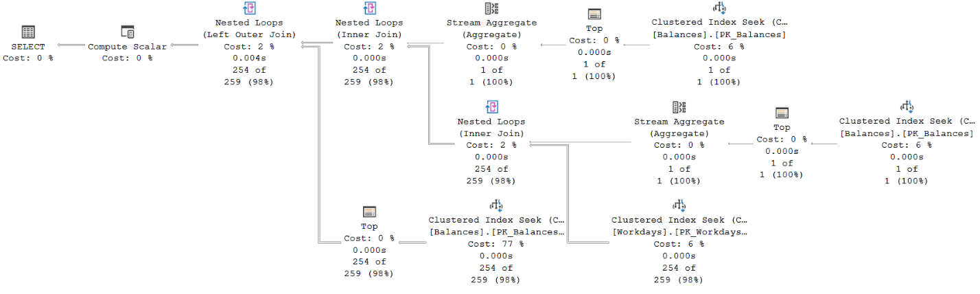
Figure 1: Plan for Solution 1
The top two seeks against the Balances clustered index obtain the minimum and maximum balance dates for the account. Each involves as many logical reads as the depth of the index (3 levels in our case). These two seeks represents a small portion of the cost of the plan (12%).
The bottom right seek against the Workdays clustered index obtains the dates of the workdays between those minimum and maximum. This seek involves just a couple of logical reads since each leaf page holds hundreds of dates, and recall that in our scenario, each account has an average of about 200 qualifying workdays. This seek also represents a small portion of the cost of the plan (6%).
The bulk of the cost of this plan is associated with the bottom left seek against the Balances clustered index (77%). This seek represents the TOP subquery obtaining the last known balance, and is executed per qualifying workday. With an average of 200 qualifying workdays and 3 levels in the index, this seek performs about 600 logical reads across all executions.
Notice that there’s no explicit sorting in the plan since the query ordering request is satisfied by retrieving the data based on index order.
Here are the performance numbers that I got for this solution in average per proc execution:
Duration with SSMS test: 698 microseconds
Duration with ostress test: 491 microseconds
Logical reads: 672
Solution 2, using IGNORE NULLS
SQL Server 2022 introduces a number of T-SQL features to support queries involving time-series data. Once specific feature that is relevant to our challenge is the standard NULL treatment clause for offset-window functions (FIRST_VALUE, LAST_VALUE, LAG and LEAD). This feature allows you to specify the IGNORE NULLS clause if you want the function to continue looking for a non-NULL value when the value in the requested position is missing (is NULL). You can find more details about the NULL treatment clause here.
Following is my second solution, which uses the NULL treatment clause:
|
1 2 3 4 5 6 7 8 9 10 11 12 13 14 15 16 17 18 19 |
CREATE OR ALTER PROC dbo.GetBalances @accountid AS INT AS SET NOCOUNT ON; SELECT W.dt, LAST_VALUE(B.balance) IGNORE NULLS OVER(ORDER BY W.dt ROWS UNBOUNDED PRECEDING) AS balance FROM dbo.Workdays AS W LEFT OUTER JOIN dbo.Balances AS B ON B.accountid = @accountid AND W.dt = B.dt WHERE W.dt BETWEEN (SELECT MIN(dt) FROM dbo.Balances WHERE accountid = @accountid) AND (SELECT MAX(dt) FROM dbo.Balances WHERE accountid = @accountid) ORDER BY W.dt; GO |
The code performs a left outer join between Workdays and Balances. It matches workday dates that appear between the minimum and maximum balance dates for the account (obtained with subqueries like in Solution 1) with the balance dates for the account. When a match is found, the outer join returns the respective balance on that workday date. When a match isn’t found, the outer join produces a NULL value as the balance.
The SELECT list then computes the last known balance using the LAST_VALUE function with the IGNORE NULLS clause.
Like in Solution 1, this solution’s code returns the data ordered by W.dt.
The plan for Solution 2 is shown in Figure 2.
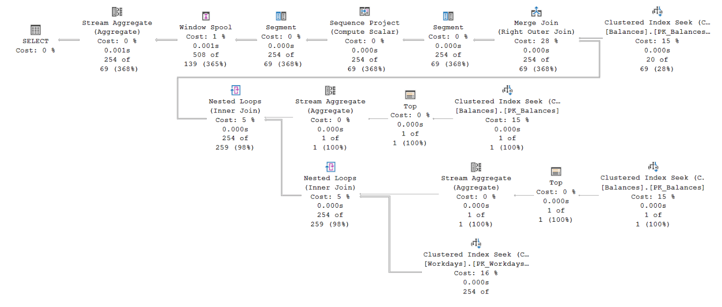
Figure 2: Plan for Solution 2
The topmost seek in the plan against the Balances clustered index retrieves the balances for the account. The cost here is 3 logical reads.
The two seeks in the middle of the plan against the Balances clustered index retrieve the minimum and maximum balance dates for the account. Each costs 3 logical reads.
The bottom seek against the Workdays clustered index retrieves the workday dates in the desired range. It costs a couple of logical reads.
The Merge Join (Right Outer Join) operator merges the workday dates with the respective balance dates based on index order, preserving the workday dates.
Finally, the operators to the left of the Merge Join operator compute the LAST_VALUE function’s result, applying the logic relevant to the IGNORE NULLS option.
Like with Solution 1’s plan, this solution’s plan has no explicit sorting since the query ordering request is satisfied by retrieving the data based on index order.
Here are the performance numbers that I got for this solution in average per proc execution:
Duration with SSMS test: 395 microseconds
Duration with ostress test: 282 microseconds
Logical reads: 11
As you can see, that’s a significant improvement in runtime and a dramatic improvement in I/O footprint compared to Solution 1.
Solutions 3a and 3b, Matching Balance Date Ranges with Workdays
The characteristics of our data are that there are very few balances per account (an average of 12.5), and many more applicable workdays (an average of about 200). With this in mind, a solution that starts with Balances and then looks for matches in Workdays could potentially be quite optimal, as long as it also gets optimized this way. Here’s solution 3a implements this approach:
|
1 2 3 4 5 6 7 8 9 10 11 12 13 14 15 16 17 |
CREATE OR ALTER PROC dbo.GetBalances @accountid AS INT AS SET NOCOUNT ON; WITH C AS ( SELECT B.dt, B.balance, LEAD(B.dt) OVER(ORDER BY B.dt) AS nextdt FROM dbo.Balances AS B WHERE accountid = @accountid ) SELECT ISNULL(W.dt, C.dt) AS dt, C.balance FROM C LEFT OUTER JOIN dbo.Workdays AS W ON W.dt >= C.dt AND W.dt < C.nextdt ORDER BY dt; GO |
The query in the CTE called C uses the LEAD function to create current-next balance date ranges.
The outer query then uses a left outer join between C and Workdays (aliased as W), matching each balance date range with all workday dates that fall into that date range (W.dt >= C.dt AND W.dt < C.nextdt).
The SELECT list returns the first non-NULL value among W.dt and C.dt as the result dt column, and C.balance as the effective balance on that date.
The outer query returns the result ordered by the result column dt.
The plan for Solution 3a in Figure 3.
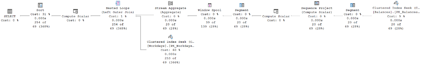
Figure 3: Plan for Solution 3a
The top seek against the clustered index on balances retrieves the balances for the account. This seek costs 3 logical reads. The remaining operators to the left of the seek and before the Nested Loops operator compute the LEAD function’s result, relying on index order. Then, a seek is applied against the clustered index on Workdays per balance date range. In average, you get 12.5 seeks, each costing a couple of reads.
The one tricky thing in this plan is that there’s a Sort operator used to handles the query’s presentation ordering request. The explicit sorting is needed since the ordering expression is a result of a computation with the ISNULL function. That’s similar to breaking SARGability when applying manipulation on the filtered column. Since we’re talking about a couple hundred rows that need to be sorted in average, the sort is not a disaster, but it does require a memory grant request, and it does cost a bit.
Here are the performance numbers that I got for this solution in average per proc execution:
Duration with SSMS test: 278 microseconds
Duration with ostress test: 211 microseconds
Logical reads: 26
Even though the number of logical reads is a bit higher than for Solution 2, the runtime is an improvement.
If we could just get rid of the explicit sorting though! There is a neat trick to achieve this. Remember, the sorting is required due to the fact that the ordering expression is the result of a computation with the ISNULL function. You can still get the correct ordering without manipulation by ordering by the composite column list C.dt, W.dt.
Here’s solution 3b implements this approach:
|
1 2 3 4 5 6 7 8 9 10 11 12 13 14 15 16 17 |
CREATE OR ALTER PROC dbo.GetBalances @accountid AS INT AS SET NOCOUNT ON; WITH C AS ( SELECT B.dt, B.balance, LEAD(B.dt) OVER(ORDER BY B.dt) AS nextdt FROM dbo.Balances AS B WHERE accountid = @accountid ) SELECT ISNULL(W.dt, C.dt) AS dt, C.balance FROM C LEFT OUTER JOIN dbo.Workdays AS W ON W.dt >= C.dt AND W.dt < C.nextdt ORDER BY C.dt, W.dt; GO |
The plan for Solution 3b in Figure 4.
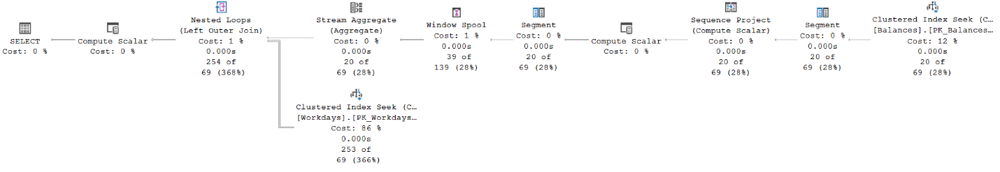
Figure 4: Plan for Solution 3b
Voila! The plan is similar to that of Solution 3a, but the sort is gone.
Here are the performance numbers I got for this solution:
Duration with SSMS test: 196 microseconds
Duration with ostress test: 165 microseconds
Logical reads: 26
That’s a pretty nice improvement compared to the performance numbers that we started with for Solution 1.
Performance Summary
Figure 5 shows the performance test results. It has the average runtimes using both the SSMS test and the ostress test summarized as bar charts corresponding to the left Y axis, and the line chart representing the average logical reads corresponding to the right Y axis.
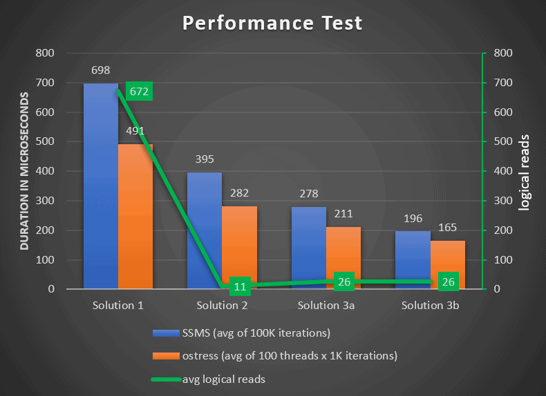
Figure 5: Performance Test Summary
Conclusion
In this article I covered a gap-filling challenge that involved gap-filling balances with missing workday dates, and for each reporting the last known balance. I showed three different solutions including one that uses a new time-series related feature called the NULL treatment clause.
As you can imagine, indexing and reuse of cached query plans were paramount here, and both were handled optimally. Using a good representative sample data that adequately represents the production environment, and an adequate testing technique are also important.
The performance expectations were for a sub-millisecond runtime in a concurrent workload, and this requirement was achieved. In fact, all solutions satisfied this requirement, with the last taking less than 200 microseconds to run.
This document contains proprietary information and is protected by copyright law.
Copyright © 2026 Red Gate Software Limited. All rights reserved
Load comments