There’s a very easy way to confuse the SQL Server query optimizer: write generic queries intended to be reused as much as possible.

Now, of course, confusing the optimizer isn’t something we generally want to do. A confused optimizer generates sub-optimal or even plain wacky execution plans. Those in turn lead to poor performance, unhappy users and late nights trying to figure out why that damn database call is timing out again.

Part of the problem is that this is another place where good software design practices for front end languages aren’t always suitable for database queries. Modern software engineering principles encourage code reuse. Code should not be written twice. If a similar task is performed in two places, the similarity should be refactored out and a function (module, method) created with the common code; a function that is then called from the two places. This is a good thing. Removing duplication reduces the chance of bugs, such as if a change is made in one place but not the other, makes maintenance easier and allows future development to be faster by providing existing building blocks.

Great, but not so great unfortunately when the same principles are applied to the database They don’t work so well in T-SQL and they’re often not compatible with how the query optimizer behaves.

And so first, a brief, high-level diversion into how the query optimizer behaves.

The Query Optimization Process

There are several references available on the internals of the query optimizer, so I’m not going to go into a huge amount of detail. Let’s just look at the high-level process.

The optimizer operates on a batch (unless there’s a recompile, but let’s ignore that for now). This means either a stored procedure, function or a set of ad-hoc statements. For the purpose of this article, I’m going to assume it’s a stored procedure, but the rules for the others are similar enough.

During the query compilation process, the stored procedure passes from the parser to the algebrizer then to the optimizer, and the latter generates execution plans for all applicable statements in the procedure, prior to any of them being executed. Control flow statements aren’t evaluated because the optimizer cannot execute T-SQL code. That means that the optimizer will still generate an execution plan for a query such as shown in Listing 1, even though the IF condition means that the query will never execute. The importance of this will be apparent later in this article.

Listing 1

To produce a good enough execution plan, the optimizer needs to know how many rows will be processed by each operator in the query. This is a problem, because the optimizer can’t run the query to determine the row count, as an execution plan is needed to run a query and the row count is needed to generate the execution plan. Instead there’s a Cardinality Estimator, which uses a whole pile of complex algorithms to estimate the row counts.

Part of what the Cardinality Estimator does is look at the constants, variables and parameters used within the queries and estimate row counts based on those values. It can see the value of parameters and constants, it cannot see the value of variables (unless there’s a recompile, but again let’s ignore that for now). This is called “Parameter Sniffing”. This is usually a good thing.

The optimization process is not performed every time the query runs. Query optimization is an expensive process and it’s only getting more expensive, as the optimizer gets smarter. Hence, SQL Server places the generated plans into the plan cache. If the query optimizer receives the same batch later, it will fetch the plan from cache instead of generating a new one.

Plans are cached with the intent to be reused, so the optimizer has to ensure that the plan is safe for reuse. That is, no matter what values are passed for parameters, the optimizer must ensure that if it uses the same plan for same batch, but executed with different parameter values, it will produce correct results.

The plan matching is done on the object id, if the batch is a procedure or function, or on a hash of the query text if the batch is ad-hoc, as well on a number of SET options. In other words, for the plan to be reused, not only must the Object ids or hashes of the query text match, but also the SET options used for each execution.

The value of the parameters is not considered when matching to a cached plan. A change in the value of the parameters will not cause the plan to be discarded and recompiled. If the values that were passed as input parameters, on initial plan creation, result in a row count that is very non-representative of the real row counts that will result from future executions of the procedure then this is the root cause of what’s called “Bad parameter sniffing”, or a “Parameter Sniffing Problem”.

Once a query plan has been generated or fetched from cache, it’s passed to the Query Processor. The Query Processor does not have the ability to reject the plan as inefficient. It cannot, if an operator in the plan is estimated to affect 10 rows, reject the plan if it’s processed 10 000 000 rows through that operator. The plan is assumed to be good enough and if it isn’t the query’s performance will suffer.

The rest of this article is going to examine coding patterns that tend to result in a generated plan or one fetched from cache that is definitely not good enough.

First up, one of my old favorites.

The Catch-all Query

The catch-all query usually looks as if it was designed by committee. “But, what if someone wants to search by the transaction amount?” or “What if someone wants to search by the date the user created the row?” and so on.

It’s characterized by a long list of parameters, most if not all optional, and a query that allows for rows to be filtered by the parameter values that are passed and to ignore the filters on parameters which aren’t passed.

Listing 2 shows one of the more common forms of this query (taken from AdventureWorks).

Listing 2

The TransactionHistory table that this query references has an index on ProductID and an index on TransactionType, both single column indexes.

Let’s look at that query, in the context of how the optimizer works, and let’s say for example, that the first execution of that procedure, the one which creates the execution plan, was with the following parameters:

• @ProductID = 42
• @TransactionType = NULL
• @Qty = 10

The index on ProductID isn’t covering, so the optimizer has to make a choice between performing a seek on the non-clustered index, and then key lookups to fetch the rest of the columns, or instead simply scanning the clustered index.

Let’s say that the estimated cardinality is low enough that the cost of the key lookups is acceptable. The optimizer would then normally produce a plan that seeks on the ProductID index with a seek predicate of ProductID = 42, does key lookups to fetch the Quantity column and does a secondary predicate on the Quantity column.

With this type of query however, it cannot do that. If the plan has a seek with a seek predicate of ProductID = @ProductID, then should the plan be reused by an execution where @ProductID is set to NULL, it will produce incorrect results. The seek predicate, the predicate determining which rows are retrieved from the index, would be an equality with NULL (ProductID = NULL), and so will return no rows.

Therefore, the plan produced typically has index scans, in this case an index scan on the ProductID index with a predicate “ProductID = @ProductID OR @ProductID IS NULL“, a key lookup to fetch the Quantity and TransactionType columns and a predicate on the key lookup of “(TransactionType = @TransactionType OR @TransactionType Is NULL ) AND (Qty = @Qty or @Qty IS NULL)“.

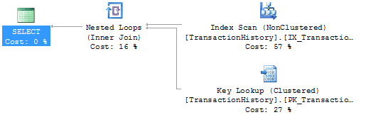
Figure 1

Figure 2 shows the Properties for the Index Scan and Key Lookup. The estimated rows are reasonably low, as would be expected since the optimizer doesn’t like doing key lookups on lots of rows. The difference between estimated and actual rows is within reason; the estimation is high because there is no Product with and ID of 42.

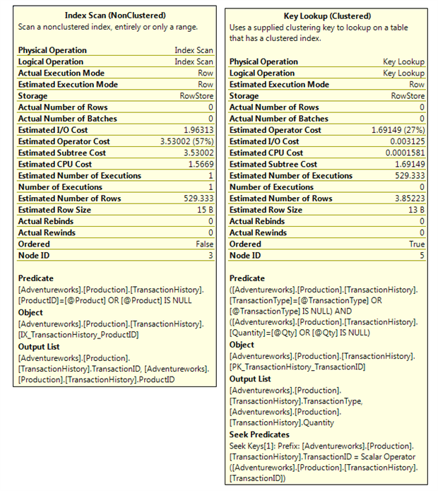
Figure 2

Now, what happens if the next call to the procedure is with the following parameter values?

• @ProductID = NULL
• @TransactionType = 'W'
• @Qty = 10

The cached plan will be reused. There’s nothing that has invalidated or removed the plan and so it will get reused.

The execution plan looks the same, which of course it has to do since it’s the cached plan which was reused, but the properties tell an unpleasant story, as shown in Figure 3.

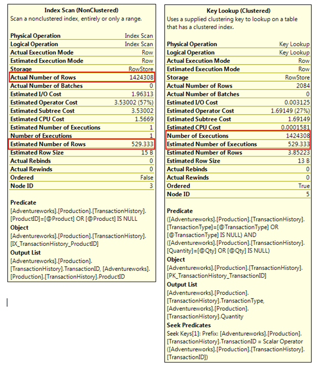
Figure 3

The index scan on the ProductID index now returns every row of the table, because if we supply NULL for @ProductID then the predicate “ProductID = @ProductID OR @ProductID IS NULL” evaluates to true for every row.

Every single row in the entire table gets a key lookup executed to locate and filter on the TransactionType and Quantity. And so the query does many times the reads that a full table scan would have required, and takes far longer and far more CPU than it did on the first execution.

The IO Statistics bear out what the execution plan properties show.

For the record, the TransactionHistory table only has 9937 pages in the clustered index so SQL Serve ends up performing over 400 times the number of logical reads it would have needed to do if it just scanned the clustered index.

That’s the major problem with this form of query. It’s not so much that it performs badly, though it does, it’s that it will perform erratically. The example I used above ran in anything from 100 ms to 3.5 seconds, depending not only on what parameter value were supplied, but also with what parameter values the plan was compiled.

So now we know the problem, what about the solution? Well there are two possible solutions, depending on version of SQL being used, the complexity of the query, the frequency at which the procedure is likely to be called, and the amount of time available to fix it.

Option 1: Recompile

This option is available from SQL Server 2008 R2 onwards. It also works in some service packs of SQL Server 2008, but has an “incorrect results” bug in others, In short, I don’t recommend using it on SQL Server 2008 unless you’ve got the latest service pack.

With the recent versions of SQL Server, putting Option (Recompile) on the statement has two effects:

1. It relaxes the optimizer’s requirement for the plan to be safe for reuse, since it will never be reused.
2. It ensures that the plan is optimal for the parameters passed on that particular execution.

Relaxing the requirement that the plan be safe for reuse means that the optimizer now can use index seek operations

Listing 3 simply adds the Option (Recompile) to the statement used in the previous example.

Listing 3

Now, for the two sets of parameters listed above, we get completely different plans, and they’re both as optimal as possible for the parameter values passed and the columns actually been searched on.

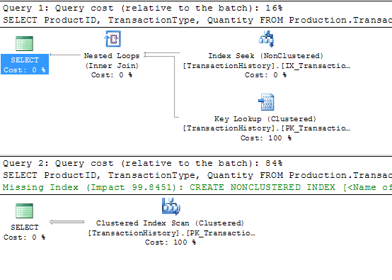
Figure 4

In the first execution, where ProductID is passed the value of 42, we now get the index seek that we initially expected. The plan no longer has to be safe for reuse, because it’s not cached and hence will never be reused. For the second execution, with TransactionType and Quantity being passed, we get a completely different plan. The cardinality estimate on the TransactionType predicate is too high for SQL to want to do an index seek and key lookups, so we get a table scan. If the index was widened to contain all the other columns the query needs, the plan would contain a seek operation on the TransactionType index.

The downside to this method is that the query has to be compiled on every execution. This probably isn’t a major concern in most cases, but it is a couple milliseconds more CPU on each execution. If the query is one which has to run hundreds of times a second or the server is already constrained on CPU, then that small CPU increase may not be desired. In that case, there’s the dynamic SQL option.

Option 2: Dynamic SQL

The second option is to use dynamic SQL. Prior to SQL Server 2008, and even in some builds of SQL Server 2008, this was the only option that worked.

These days, dynamic SQL represents a more complex, harder-to-read way of solving the problem than using the Recompile hint. In fact, since SQL Server 2008 R2 became prevalent, I’ve used the dynamic SQL solution only once, for a query that was running many times a second.

That’s said, let’s see how it works.

Using the dynamic SQL solution, we build up a WHERE clause string containing only those predicates that correspond to the parameters that were passed with a value. If the TransactionType was not passed, if the parameter was NULL, then the string we send for execution contains no filter on TransactionType.

It is also critically important when using dynamic SQL that you don’t accidentally introduce a SQL Injection vulnerability. Never concatenate a parameter directly into the string that is to be executed. Instead, use the sp_executesql procedure to pass parameters to the dynamic SQL. Therefore, what gets executed is a parameterized SQL statement.

Listing 4

It’s a little, well no it’s a lot more complicated than the Recompile option, so let’s examine it one section at a time.

The first couple of statements are easy enough; they’re just declaring variables and setting up the portion of the SELECT that doesn’t depend on the parameters passed. In some cases, this string may include WHERE clause predicates, if there are predicates which are always evaluated.

The second section sets up the conditional portions of the WHERE clause. It’s important to notice that I am at no point concatenating parameters into the @sSQL dynamic SQL string. Instead, the parameters are used to decide what string fragments to include in the WHERE clause of the dynamic SQL string. Those WHERE clause predicates are parameterized and when we execute that dynamic SQL statement, the inner parameters will have values passed to them.

The third part is the way I choose to handle adding the built up WHERE clause to the rest of the query, by removing the AND from the first clause. The alternative is to use the “WHERE 1=1 AND...” construct, which I hate with a passion.

Finally we execute the query. The procedure sp_executeSQL has three parameters. The first is the statement to be executed, of type NVARCHAR. The second is the list of parameters that appear in the dynamic SQL, with their data types. It’s perfectly acceptable to define parameters which aren’t used in the dynamic SQL, which is why the parameter list is not also defined by the values passed to the procedure. The third is where the defined parameters are given their values.

That’s the setup of the dynamic SQL, now let’s see how it behaves when we execute it. As in the previous examples, I’m going to execute two calls to the procedure.

The first call passes in ProductID and Qty parameters only, and Figure 5 shows the execution plan.

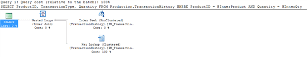
Figure 5

The plan is the same as the one we saw for the equivalent call to the code containing OPTION(RECOMPILE). The difference here is that the query has no reference to TransactionType at all; the WHERE clause contains only the two predicates that were passed. Similarly, the second call passing in only TransactionType and Qty shows a query which only has those two predicates and again the execution plan shows a clustered index scan.

All well and good, but how do they perform?

To answer that, I cleared the plan cache and then ran each of the following 10 times and averaged the performance:

• Catch-all original code with ProductID and Qty parameters passed
• Catch-all original code with TransactionType and Qty parameters
• Recompile option with ProductID and Qty parameters passed
• Recompile option code with TransactionType and Qty parameters
• Dynamic SQL option with ProductID and Qty parameters passed
• Dynamic SQL option code with TransactionType and Qty parameters

Figure 6 summarizes the results.

Variation	Parameters passed	Average CPU (ms)	Average duration (ms)
Original	ProductID, Qty	97	98
	TransactionType, Qty	2561	2572
Recompile	ProductID, Qty	3	2
	TransactionType, Qty	76	78
Dynamic SQL	ProductID, Qty	0	0
	Transactiontype, Qty	72	75

Figure 6

That, I think, wraps up the catch-all query. Next on the list of tricks to confuse the optimizer, the problems that control flow can cause.

When Control Flow Attacks

By control flow, I’m talking mostly about the IF keyword. You can achieve similar behavior with a WHILE loop, but it’s a hell of a lot less likely (typically WHILE is used to repeat code, such as INSERTs, rather than decide which blocks of code will execute at all), and WHILEtends to be far less common in T-SQL code than IF, at least in code I see.

What, though, can cause problems when there’s control flow statements? Let me repeat two things I said in the brief description of the optimization process:

“The optimizer gets the stored procedure and generates execution plans for all applicable statements in the procedure. Control flow statements aren’t evaluated.”

“Part of what the Cardinality Estimator does is look at the constants, variables and parameters used within the queries and it will estimate row counts based on those values.”

The first time the procedure runs, all queries in the procedure get optimized, regardless of control flow statements, and the queries get optimized based on the parameters passed to the procedure on that first execution. That means that a query inside an IF blocks may be compiled based on parameter values with which it will never execute.

If, for example, we had the following in a procedure:

We can see that if 0 has been passed as @Param, then the query cannot execute. However, if the first execution of that procedure was with @Param = 0, then the optimizer would still generate an execution plan for that query based on the parameter value @Param = 0.

Let’s look at an example. We have customer and order tables and let’s say there’s a search screen in the app that allows users to locate customer’s orders either by order number or by status, but not by both. Hence, this isn’t another catch-all query. A typical stored procedure to implement this logic might look something like that shown in Listing 5.

Listing 5

Let’s say that the first execution passes @AccountNumber and @OrderNumber but leaves @OrderStatus at its default.

What happens when the procedure is compiled? The optimizer encounters the query that filters by OrderNumber and generates a plan based on the value of @OrderNumber that was passed. Fine, so far. Next the optimizer encounters the query that filters by OrderStatus and optimizes it for a parameter value of NULL. That is, it optimizes the query based on the WHERE clause predicate OrderStatus = NULL. This is a problem.

It’s a problem because, unless ANSI_NULLS is at a non-default and deprecated setting (very rare), then the predicate OrderStatus = NULL must return zero rows, as nothing is ever equal to NULL.

Therefore, the procedure’s plan goes into cache with the first query optimized based on the parameter value with which it ran, and the second query optimized based on a parameter value with which it can never run, because of the IF statement.

If we look at the actual plan for the first execution, we only see the plan for the query which ran on that execution.

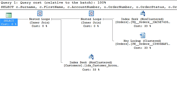
Figure 7

So was I wrong earlier when I said all queries in the procedure are optimized on first execution? No, this is another case where Management Studio is lying. Let’s pull the cached plan and see what it looks like.

Listing 6

Figure 8 shows the plan.

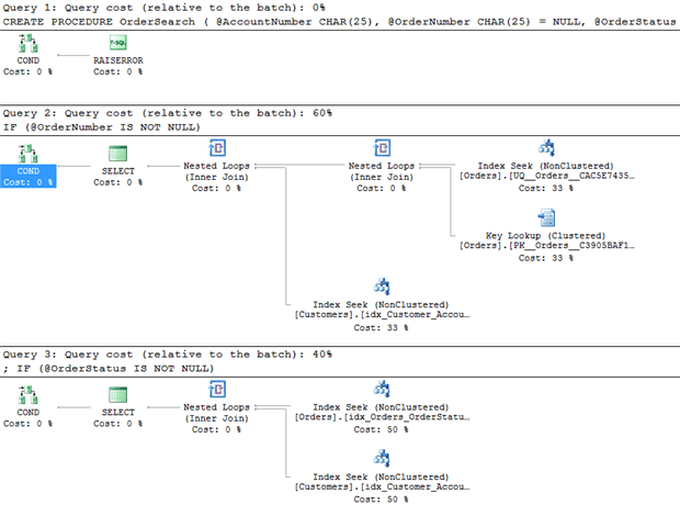
Figure 8

The cached plan does indeed have both queries in it, with conditionals as the first operators. The conditional is the plan operator for the IFs and they get executed first. Only if the conditional evaluates to true does the rest of the plan get executed.

Now let’s see what happens when, with the above plan in cache, we run the procedure and pass a value for @OrderStatus only, rather than @OrderNumber only.

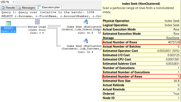
Figure 9

Estimated rows 1, actual rows just over 4 million. That’s really going to mess up the optimizer. That’s 4 million rows feeding into the Nested Loops join. The Nested Loops will execute the inner portion of the join, the index seek on Customers, once for each row coming from the outer index seek, the one on Orders. That’s 4 million index seeks against the Customers table.

The one row estimate is because the plan was compiled with a parameter value of NULL, a parameter that would result in the query returning 0 rows.

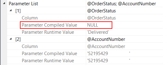
Figure 10

The execution characteristics don’t make for pleasant reading either.

It tool 10 seconds of execution, and read 63 GB of data from the Customers table. For contrast, a table scan of the Customers table reads 138 pages, or just over 1MB of data. The high logical reads is because SQL read each page in the table multiple times during the 4 million executions of the index seek against the Customers table.

Let’s clear the plan cache and run the procedure again, this time passing a value for AccountNumber and OrderStatus, and leaving OrderNumber as NULL.

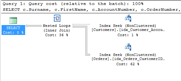
Figure 11

We still have a Nested Loops join, but the order of tables has switched. The Customers table is now the outer table for the join. This index seek returns one row. The nested loop hence runs once and runs a single seek against the Orders table. The performance characteristics show a much reduced duration and much lower reads

300ms vs 10 seconds, and most of that 300ms is from the time taken to display the records.

With the cause and effects of the problem explained, the next question is how to fix it. There are a number of options.

Option 1: Recompile

Since the problem is due to a cached plan being executed with row counts very different to the ones for which the plan was compiled, one option is to add the OPTION (RECOMPILE) hint to the end of each of the queries. This is a simple fix, it works, but it’s not the one I prefer. There are other easy ways to fix this without throwing away the ability to cache execution plans for the procedure.

If we were to use this option, the procedure would look something like as shown in Listing 7.

Listing 7

Option 2: Optimize For

Another possible solution is to use the OPTION (OPTIMIZE FOR <value>) hint on the queries. The problem is caused by the optimizer optimizing the query based on inappropriate values, so if we can specify what values the optimizer must use when optimizing the query, then we can eliminate this problem.

This option relies on being able to identify the best parameter value, one that will generate good execution plans. That’s a bit more work than using the OPTION (RECOMPILE) solution and requires that the procedure be checked as data changes to ensure that the values in the hints are still the best. This is also not my favorite solution, because I prefer to reserve hints for when I can’t solve the problem in any other way.

However, if we were to use this option, the procedure would look something like as shown in Listing 8.

Listing 8

Option 3: Break the procedure into multiple sub-procedures

The core problem is that queries are being compiled with parameter values with which they will never run. To avoid that, we can split up the single procedure into three procedures, the outer one containing the control flow and the other two procedures each containing one of the two queries.

A procedure is only compiled when it’s called, if there’s no plan already in cache for it, and plans are per-procedure, so doing this will allow each of the SELECT statements to have a cached execution plan that is optimal for the values with which the query will be executed, without resorting to any hints.

I prefer this solution where it is possible. It avoids hints and allows SQL Server to cache plans optimal for the queries. Plus, we now have ‘single responsibility’ procedures i.e. procedures that do one thing and one thing only, which is always a good idea.

Fixed in this way, the procedures would look as shown in Listing 9.

Listing 9

With three solutions discussed, let’s test them out and see how they perform compared to each other and compared to the original. As in the previous section, I ran each version of the procedure 10 times with the first set of parameters, 10 times with the second set of parameters and average the CPU and duration for each set of 10 executions.

Variation	Parameters passed	Average CPU (ms)	Average duration (ms)
Original	AccountNumber, OrderNumber	0	0
	AccountNumber, OrderStatus	10592	10587
Recompile	AccountNumber, OrderNumber	1	2
	AccountNumber, OrderStatus	27	30
Optimize for	AccountNumber, OrderNumber	0	0
	AccountNumber, OrderStatus	25	28
Sub	AccountNumber, OrderNumber	0	0
	AccountNumber, OrderStatus	25	28

Figure 12

The performance of the second and third options are identical and the recompile is negligibly slower, so unless the procedure is running thousands of times a second, the choice of which to use comes down to personal preference.

That’s the second of the three scenarios I’m covering. Onwards!

Changing Parameter Values

A.k.a. Playing ‘Bait and Switch’ with the Optimizer

The idea here is that NULL is passed as a parameter, then the parameter value is changed to something that would allow any value to be returned. This is not a common technique but I’ve seen it used a couple of times to create a ‘generic’ procedure.

As an example, a string parameter might be set to '%' if it is passed as NULL and then the predicate that the parameter is used in is a LIKE statement.

Why is this a problem? Again, let’s reconsider the two previous statement from my initial explanation of optimization:

“Part of what the Cardinality Estimator does is look at the constants, variables and parameters used within the queries and it will estimate row counts based on those values.”

“The optimizer gets the stored procedure and generates execution plans for all applicable statements in the procedure, prior to any of them being executed.”

The optimizer generates plans based on the parameter values that are passed. If the parameter values are changed in the procedure before the query executes, the query will execute with a value for which it was not optimized.

Let’s see how this works via a simplified second-hand car search. The procedure shown in Listing 10 accepts minimum and maximum price, minimum and maximum kilometers and the make of car. All parameters are optional.

Listing 10

Let’s see how that performs. Unlike the previous examples, I don’t need to run a couple different parameter sets to show the bad behavior; this just needs one.

There is a covering index on the Make column, so in theory this call should be a straight index seek. However, that’s not what the optimizer chooses.

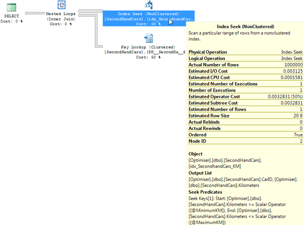
Figure 13

Instead, we see an index seek on a non-covering index, on the Kilometers column. This index seek returns every single row in the table, all 1 million of them, and performs look up for each row.

Not pretty.

Why did it pick that index? The ‘Estimated rows = 1‘ gives a good clue. A look at the parameters of the SELECT operator shows why that was the estimate.

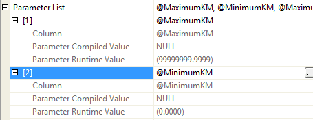
Figure 14

The two parameters used against the Kilometer column were NULL at the point the plan was compiled. At this point, I don’t think I need to go into how many rows will be returned by the predicate “Kilometers BETWEEN NULL AND NULL” We’ve seen that already.

Therefore, the optimizer generates a row estimation for a seek of 1 row, on the Kilometers index. That would take 2, maybe 3 logical reads. It could then do a lookup to the clustered index (in case there was a row), to fetch the rest of the columns and apply the other predicates. That would also be 2 or 3 reads, making it more efficient than reading the Make index. Had it done a seek on the Make index, it would have had to read all the rows for one make, and apply a secondary predicate on each one for the predicates on Kilometers and Price, and it estimated that those secondary predicates would filter out all rows.

Unfortunately, because the estimations are wildly inaccurate, searches on Kilometer are going to be highly inefficient.

Let’s discard the cached plan and call the procedure again, passing the min and max kilometers as the only parameters.

This time we get a plan seeking on the Price index, which is not covering, and again looking up all rows in the table.

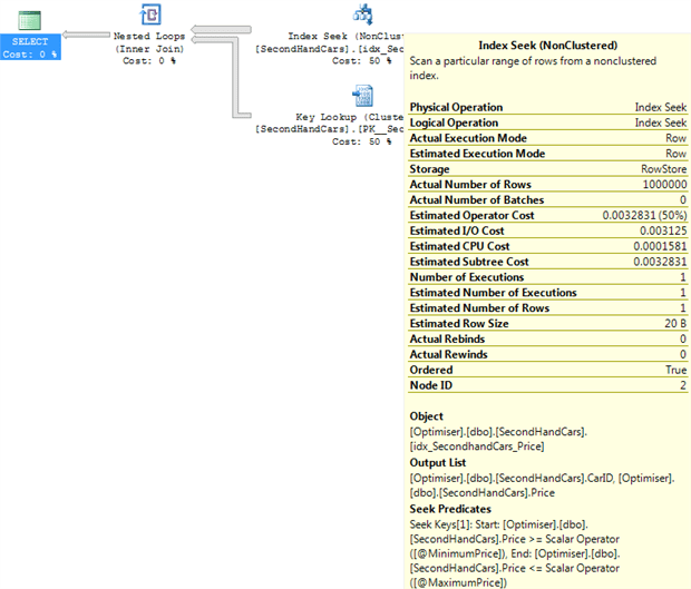
Figure 15

The execution statistics are as follows:

Because the unpassed parameters default to NULL, and because any comparison with NULL, other than IS [NOT] NULL, return no rows, the optimizer will pick an index on a column that did not have a parameter value passed for it, ensuring the worst possible plan for the parameter values with which the query is executed.

So how can we write this form of procedure efficiently? Again there are multiple options.

Option 1: Dynamic SQL

The dynamic SQL option solution looks much the same as the dynamic SQL solution for the catch-all query. Only the parameters passed with a value are used to form the WHERE clause, and so the dynamic SQL query constructed only has the predicates which will actually filter the resultset. Each different piece of dynamic SQL gets a different plan (it’s compiled as an ad-hoc plan rather than as part of the procedure’s plan)

I’m not going to explain the dynamic SQL here, it’s all explained in the earlier section on catch-all queries. The procedure using dynamic SQL will look as shown In Listing 11.

Listing 11

This is not my preferred solution. Much as with the catch-all query, while the dynamic SQL solution works fine, it’s overly complicated.

Option 2: Use sub-procedures

Since the problem is that a procedure is being called with parameter values with which the query will never be executed, one option is to change the parameter values in an outer procedure and then call a sub-procedure. Since there are no queries in the procedure where the parameter values are being changed, and since the unit of compilation is the procedure, there’s no longer any way for queries to be executed with parameters whose values changed between compilation and execution.

This is a solution which may work in some circumstances, but could result in a procedure that is prone to traditional parameter sniffing problems if it is a search procedure like the one I’ve used as an example. Searching for @MinimumKM = 20000, @MaximumKM = 25000 vs searching for @MinimumKM = 0, @MaximumKM = 500000 will have very different row counts, making the procedure susceptible to classic bad parameter sniffing. For completeness, Listing 12 shows the code for this solution but please evaluate it carefully before using it, in case one of the other solutions is more appropriate.

Listing 12

Option 3: Recompile

My preferred solution, and the simplest solution, is to add OPTION (RECOMPILE) to the query. Firstly, this fixes the problem of the query being compiled with parameter values with which it will never run, and second it ensures that there’s no chance of a bad parameter sniffing problem, as there is in option 2.

With OPTION (RECOMPILE), the optimizer generates the plan based on the parameter values passed each time the queries within the procedure run, rather than just the first time we execute the procedure. Furthermore, the plan is not cached.

As with the catch-all query, unless the procedure runs many, many times a second or the server is constrained on CPU, there shouldn’t be any concerns about this option.

Listing 13

On to the testing. As previously, I’m going to run each version of the procedure 10 times. I’m first going to run the procedures with only the Make parameter passed, then, without clearing the cache, with just the min and max kilometer parameters, then with the make and max price parameters.

Variation	Parameters passed	Average CPU (ms)	Average duration (ms)
Original	Make	2303	2312
	MinimumKM, MaximumKM	270	273
	Make, MaximumPrice	2104	2106
Dynamic SQL	Make	42	42
	MinimumKM, MaximumKM	139	144
	Make, MaximumPrice	25	28
Sub procedures	Make	69	68
	MinimumKM, MaximumKM	315	316
	Make, MaximumPrice	42	43
Recompile	Make	69	69
	MinimumKM, MaximumKM	318	324
	Make, MaximumPrice	42	45

Figure 16

In this test, the dynamic SQL solution came out ahead, because only filtering on the criteria that will actually reduce the row count means that the optimizer can choose more efficient indexes. The sub procedure worked well here, but may not work as well in all circumstances, so testing is required. The recompile came in the worst of the three solutions, by a small margin due to the compilation overhead on every execution, though this has to be weighed against the ease of implementation.

Conclusion

The moral of this article is that if you really want to confuse the query optimizer, feed it generic, ‘reusable’ SQL. We’ve examined three common forms of generic SQL: catch-all queries, use of control flow to create general purpose stored procedures, and switching parameter values within a procedure. These aren’t the only forms that exist, but they are the ones I see most often.

These techniques will cause the optimizer make wildly inaccurate assumptions regarding the selectivity of a particular predicate, often based on parameter values with which the query could never execute. This results in the creation and reuse of very sub-optimal execution plans and therefore in slow queries, or queries that are infuriatingly erratic in their performance.

We looked at the most common options for optimizing the performance of this sort of code, such as recompiling the query on each execution, using hints, dynamic SQL, or splitting generic procedures into sub-procedures.

Each of these techniques can be made to work, but all have certain drawbacks. In SQL Server, generic code is often slow code. Avoid it if you possibly can.

(DDL Download: ftp://ftp.simple-talk.com/articles/GailShaw/Optimizer.zip )