
I spend a lot of time on the SQLServerCentral, and other SQL community forums, trying to help SQL Server users who find themselves in difficulties. Over time, I’ve seen certain misunderstandings and mistakes occur with alarming regularity. Here I pick just four of my “favorite” SQL Server howlers, covering misunderstanding of partitioning, misguided index strategies, abuse of hints, and the never-ending quest for “go-faster” server settings.
Missing the Point of Partitioning
“I partitioned my table, but my queries aren’t any faster…!”
Partitioning is a feature that’s mostly intended to aid in maintenance on larger tables and to offer fast ways to load and remove large amounts of data from a table. Partitioning can enhance query performance, but there is no guarantee.
Partitioning and Query Performance
Let’s look at a textbook example, the Orders and OrderDetails tables for a hypothetical internet vendor.
|
1 2 3 4 5 6 7 8 9 10 11 12 13 14 15 16 17 18 19 20 |
CREATE TABLE Orders ( OrderID INT IDENTITY NOT NULL, OrderDate DATETIME NOT NULL , CustomerID INT NOT NULL , -- foreign key to customers OrderStatus CHAR(1) NOT NULL DEFAULT 'P' , ShippingDate DATETIME ); CREATE TABLE OrderDetails ( OrderID INT , OrderLineID INT , OrderDate DATETIME , -- there is a reason this is in the detail -- as well as the header ProductID INT , -- foreign key to products OrderQuantity INT , LineTotal MONEY ); |
Listing 1: The Orders and OrderDetails tables
This is simple enough; in the script, PartitionTableDefinition.sql (available for download at the bottom of the article), I create two copies of those tables, one to be partitioned and one to be left un-partitioned.
I’m going to partition the table on the OrderDate column, which is a fairly logical and normal choice for this kind of table, given that many queries will be likely filtering by date, and has the advantage that the column is reasonably narrow, unchanging and ascending, all desirable attributes for the clustered index.
Listing 2 shows the partition schema and function. We create seven partitions (Partition1 for any dates earlier than 2011/11/01, Partition2 for 2011/11/01 up to 2011/11/30, and so on), all of which, in this example, I’m mapping into the PRIMARY filegroup, simply because I don’t have extra drives to split them across. However, for reasons we’ll discuss later, this is unlikely to have too much of an impact in this case.
|
1 2 3 4 5 6 7 8 |
CREATE PARTITION FUNCTION PartitionByMonth (DATETIME) AS RANGE RIGHT FOR VALUES ('2011/11/01', '2011/12/01', '2012/01/01', '2012/02/01', '2012/03/01', '2012/04/01'); CREATE PARTITION SCHEME PartitionToPrimary AS PARTITION PartitionByMonth ALL TO ([PRIMARY]); |
Listing 2: Creating the partition function and partition scheme
I use the same partition schema and function for both tables, which is the reason why the OrderDetails table has an OrderDate column in it, a column that shouldn’t really be in there as it is an attribute of the order, not the order line items. Still, if I’m going to partition both by date, they both need the date column in them. With our partitioning in place, Listing 3 creates the necessary indexes for each of our tables.
|
1 2 3 4 5 6 7 8 9 10 11 12 13 14 15 16 |
CREATE CLUSTERED INDEX idx_Orders_OrderDate ON Orders (OrderDate); ALTER TABLE Orders ADD CONSTRAINT pk_Orders PRIMARY KEY (OrderID, OrderDate); CREATE NONCLUSTERED INDEX idx_Orders_CustomerID ON Orders (CustomerID); CREATE NONCLUSTERED INDEX idx_Orders_OrderStatusOrderDate ON Orders (OrderStatus, OrderDate); CREATE CLUSTERED INDEX idx_OrderDetails_OrderDate ON OrderDetails (OrderDate); ALTER TABLE OrderDetails ADD CONSTRAINT pk_OrderDetails PRIMARY KEY (OrderID, OrderLineID, OrderDate); CREATE NONCLUSTERED INDEX idx_OrderDetails_ProductID ON OrderDetails (ProductID); GO |
Listing 3: Primary keys and Indexes
The next step is to populate each table. In the provided script, I load 500,000 rows per month for 6 months into the Orders table (for a total of 3 million rows) and 2,000,000 rows per month for 6 months into the OrderDetails table (for a total of 12 million rows).
We’re now ready to try some simple queries to see how the two tables (partitioned vs. un-partitioned) perform. The unwary developer tends to expect a performance improvement in the partitioned queries that is proportionate to the portion of the table that the queries can ignore. For example, if the table has 6 months of data and is partitioned by date and then we query and filter for only the one month of data, then SQL can ignore 5/6 of the data in the table and hence they expect that the query should be of the order of 6 times faster.
|
1 2 3 4 5 6 7 8 9 10 11 12 13 14 15 16 17 18 19 20 21 22 23 24 25 26 27 28 |
-- Query 1: Total per customer for the last month SELECT CustomerID , SUM(LineTotal) AS TotalPurchased FROM dbo.Orders AS o INNER JOIN dbo.OrderDetails AS od ON o.OrderID = od.OrderID WHERE o.OrderDate >= '2012/04/01' GROUP BY CustomerID -- Query 2: Total per product for one month SELECT ProductID , SUM(OrderQuantity) FROM dbo.OrderDetails AS od WHERE OrderDate >= '2011/12/01' AND OrderDate < '2012/01/01' GROUP BY ProductID -- Query 3: Which customers bought product X? SELECT DISTINCT CustomerID FROM dbo.Orders AS o INNER JOIN dbo.OrderDetails AS od ON o.OrderID = od.OrderID WHERE ProductID = 375; -- Query 4: Are any orders unshipped for more than 2 months? SELECT OrderID FROM dbo.Orders AS o WHERE OrderDate < DATEADD(mm, -2, '2012/05/01') AND ShippingDate IS NULL; |
Listing 4: Simple queries to test partitioning performance boost
I ran each test several times, and ignored the results from the first execution (because of the cost of compiling the query and caching the data). This is the reason why the fact that the files were all in the same filegroup, on the same drive, did not affect these results; all of the reads are logical reads, reads done from memory, not from disk. On larger, less-used tables, if multiple partitions were going to be read and the data was not in memory, then having the tables partitioned and the partitions on different IO paths might provide a performance benefit.
I aggregated the results from a Profiler trace, and Table 1 shows the average CPU, and average number of reads, for each pair of queries against the partitioned and un-partitioned tables.
| Query | Average CPU | Average Reads |
| Query 1 Partitioned | 2302 | 73337 |
| Query 1 Un-partitioned | 2704 | 75565 |
| Query 2 Partitioned | 992 | 12121 |
| Query 2 Un-partitioned | 844 | 12209 |
| Query 3 Partitioned | 272 | 50323 |
| Query 3 Un-partitioned | 232 | 63952 |
| Query 4 Partitioned | 438 | 8645 |
| Query 4 Un-partitioned | 369 | 8747 |
Table 1: Comparing query performance for partitioned and un-partitioned tables
For every query, we can see that the ones against the partitioned tables show a slightly lower number of reads, the reduction ranging from 0.7% up to 20%. The latter value is good, but it’s not phenomenal. If I were performance tuning a problematic query, I certainly wouldn’t consider a 20% reduction in reads a success. The effect on the CPU time is minimal, and in three cases, the average CPU time increases for the partitioned table. In other words, just by partitioning these two tables, we have not achieved a good improvement in the performance of these queries.
Of course, I’m not implying that partitioning never improves query performance. It certainly can do so, but it requires specific query forms, and a lot of the benefit comes from parallelizing over the partitions or, if the query is IO-bound, from additional IO bandwidth, arising from having partitions that are accessed in parallel on separate IO channels.
However it is not, for reasons that relate to index architecture, a general-purpose tool that will guarantee an easy, immediate and significant increase in query performance. Figure 1 offers a simplified depiction of index architecture for an un-partitioned table with the clustered index on a date column (a real index would have a lot more pages at the leaf level).
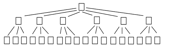
Figure 1: Un-partitioned table, 3-level deep clustered index
Let’s say that we filter for one month of data (and assume that the data is evenly distributed by month). SQL locates this data by navigating down the b-tree from the root page to the start of the range and then reads along the leaf level to the end of the range, as shown in Figure 2.
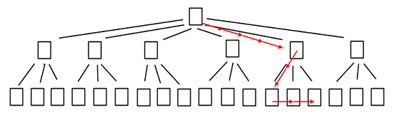
Figure 2: Navigating the un-partitioned clustered index to find the required rows
That takes five page reads: the root, one intermediate page and the three leaf pages (again, there would be far more in a real index). Now let’s compare that against a table that’s partitioned by month into six partitions, as shown in Figure 3.
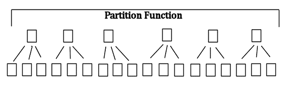
Figure 3: A table partitioned into six partitions
A partitioned table is really a collection of tables (as many as there are partitions) that behave as a single table. Each partition has its own smaller b-tree for the clustered index on that partition. Any partition-aligned non-clustered indexes are also essentially multiple smaller non-clustered indexes, one on each partition. In order to locate one month of data, the partition function tells SQL what partition holds the requested data, then it’s just a seek down the b-tree of the partition that contains the data, as shown in Figure 4.
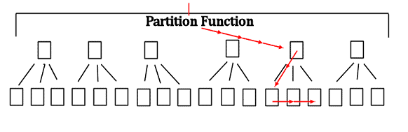
Figure 4: Navigating the partitioned clustered index to find the required rows
We haven’t avoided the need to scan the table, because with a clustered index on the date column we would never have scanned the table anyway.
So what’s the point of partitioning at all?
Partitioning and the Sliding Window Technique
The main benefits of partitioning are in maintenance and data loads. With partitioning, we can add data to, or remove it from, a huge table very easily, just by switching partitions in or out. This is termed “sliding window”, and at a high-level it works as shown in the following series of figures.
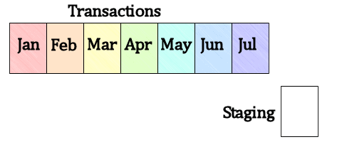
Figure 5: A partitioned Transactions table and Staging table
What we see, in Figure 5, is a table storing transactions (for example sales transactions). The table is partitioned by month and data is loaded into it at the end of each month. The Staging table has exactly the same indexes as the partitioned table, and all indexes on the partitioned table are partition-aligned (created on the same partition scheme).
To load the latest month of data into that table and remove the oldest, we can load the Staging table with the most recent data (if it’s not already loaded, say by the application) and split the most recent partition in the sales table, so that there is an empty partition at the ‘end’ of the table, as shown in Figure 6.
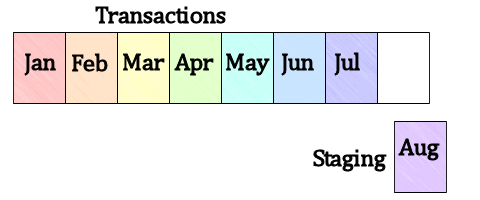
Figure 6: Load the Staging table with new data; split the most recent partition in the main table
Next, with a purely metadata operation, we can switch the Staging table with the empty partition, and the data in the Staging table is now in the main table. Since a metadata operation does not require moving the actual, rows, just changing some pointers in the system catalogs and allocation structures, this is both exceedingly fast and logs very little. It also does not require the long-duration exclusive locks that inserting into the table would require.
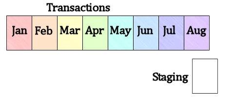
Figure 7: Switch the Staging table with the empty partition
In order to remove the oldest data from the table, we simply reverse the process. We switch the oldest partition with the empty Staging table, as shown in Figure 8.
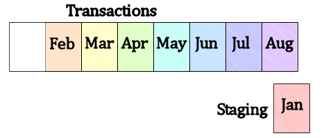
Figure 8: Switch the oldest partition with the Staging table
Then, we merge the oldest partition with the next oldest and truncate the Staging table.
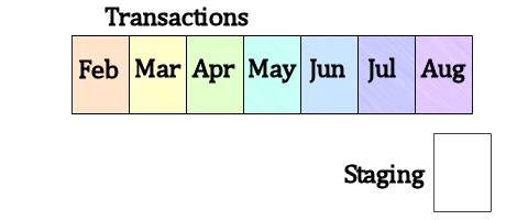
Figure 9: Merge in the empty partition, truncate the Staging table
Using this sliding window technique, we can add a million or so rows to the table, and remove another million or so rows, in milliseconds with minimal impact on the transaction log and without needing long-duration locks on the main table that could block other queries.
Using the Orders table from our previous example, our sliding window scheme would look something like as shown in Listing 5.
|
1 2 3 4 5 6 7 8 9 10 11 12 13 14 15 16 17 18 19 20 21 22 23 24 25 26 27 28 29 30 31 32 33 34 35 |
CREATE TABLE Orders_Staging ( OrderID INT IDENTITY NOT NULL PRIMARY KEY , OrderDate DATETIME NOT NULL , CustomerID INT NOT NULL , -- foreign key to customers OrderStatus CHAR(1) NOT NULL DEFAULT 'P' , ShippingDate DATETIME ); -- Create all indexes to match the partitioned orders table CREATE CLUSTERED INDEX idx_Orders_OrderDate ON Orders_Staging (OrderDate); ALTER TABLE Orders_Staging ADD CONSTRAINT pk_Orders PRIMARY KEY (OrderID, OrderDate); CREATE NONCLUSTERED INDEX idx_Orders_CustomerID ON Orders_Staging (CustomerID); CREATE NONCLUSTERED INDEX idx_Orders_OrderStatusOrderDate ON Orders_Staging (OrderStatus, OrderDate); -- add a new partition value to the partition function ALTER PARTITION FUNCTION PartitionByMonth() SPLIT RANGE ('2012/06/01') -- switch the staging table with the last partition of the Orders table. -- After this the staging table is empty and the data that was in it is -- in the Orders table ALTER TABLE Orders_Staging SWITCH PARTITION 1 TO Orders PARTITION 7 -- switch the first partition of the Orders table with the staging table ALTER TABLE Orders SWITCH PARTITION 1 TO Orders_Staging PARTITION 1 -- remove the earliest boundary point in the partition function ALTER PARTITION FUNCTION PartitionByMonth() MERGE RANGE ('2011/11/01') |
Listing 5: Implementing a sliding window for the Orders table
In terms of easing maintenance, we can rebuild individual partitions (offline only) without affecting the rest of the table. The different partitions can even have different compression settings, so we can tailor the setting as appropriate for the various usage patterns, typically with the older data getting more compression than the current data.
In addition, we can map partitions containing older, less-frequently used data to filegroup placed on slower storage, because it is not as important as the latest data, which would likely be in a partition on fast storage.
In summary, partitioning is mostly for improved maintenance, fast loads, fast deletes and the ability to spread a table across multiple filegroups; it is not primarily for query performance.
Poor Index Design
“I have indexes on all the columns in the WHERE clause, but SQL is still doing a scan…!”
This is a fun one…there are a couple of reasons why a query may scan indexes, or the table, even when there is an index that appears to support the particular query.
The most common causes are as follows:
- Index is neither sufficiently selective nor covering
- Index columns are in the wrong order to support the query
- Query predicate is not SARGable
I’ll briefly touch on each of these.
Index is insufficiently selective or not covering
For SQL Server to use an index for the evaluation of a query, one of two criteria needs to be true: the query needs to retrieve a small portion of the table, or the index needs to be a covering index.
A covering index is one where all the columns needed by the query are somewhere in the index. See http://www.simple-talk.com/sql/learn-sql-server/using-covering-indexes-to-improve-query-performance/ for further details on covering indexes.
When I say small portion of the table, I’m not talking half or a quarter or even 10%; the usual point where SQL Server will consider that a query is returning too much data to use a non-covering index is about 0.5% of the table. As a rough estimate, the cut-off point is the point where the number of rows returned exceeds 30% of the total number of pages in the table.
The reason for this cut-off is the expense of performing key lookups to retrieve the data not contained in the index, as shown in Figure 10.
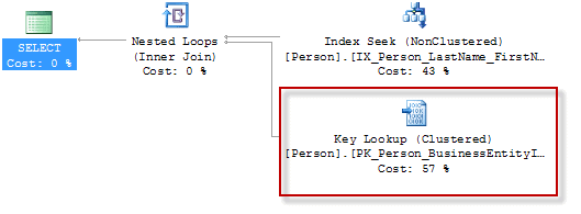
Figure 10: The costly Key Lookup
Let’s take an example query against a made-up table, and assume we have a non-clustered index on the Location column only.
|
1 2 3 4 |
SELECT FirstName , Surname FROM Customers WHERE Location = 'Tweebuffelsmeteenskootmorsdoodgeskietfontein' |
Listing 6: Find customers located in “Twee Buffels”
Now it’s unlikely that many people live in “Twee Buffels”, so SQL Server can perform a seek operation on the index and fetch the rows that match that location.
Since the index is just on the Location column, all that SQL will be able to get back from the index is the Location column, and a pointer to the row in the base table (the pointer will be either the clustered index key or a physical RID). Having retrieved the rows from the index, SQL will then do lookups to the base table to fetch the rest of the required columns. SQL Server performs these lookups one row at a time.
If we assume that the query returns three rows, SQL has to do four separate data access operations to run that query, one seek on the non-clustered index and then three lookups to the base table, one lookup for each row returned by the seek. It’s easy to see that these lookups become very expensive when a query returns many rows.
If we reran the same query with a location that returns 100,000 rows that would be 100,001 separate data accesses, each reading one or more pages (each lookup does a number of reads equal to depth of the clustered index tree, if the table has a clustered index, or one read if the base table is a heap).
It’s for this reason that SQL Server will choose not to do key lookups if the query returns a large number of rows; instead, it will perform a single scan of the whole table, which can very easily be more efficient in terms of IO than many, many, many single-row lookups
Another common cause of SQL Server choosing to scan is a query that contains multiple predicates, when no single index exists that has all the columns necessary to evaluate the WHERE clause. For example, an index on (FirstName, Surname), would fully support any query with a WHERE clause of FirstName = @FirstName AND Surname = @Surname. However, if there was one index on FirstName only, and a second separate index on Surname, then SQL Server can use neither one efficiently. It may choose to seek one index, do lookups for the other columns and then do a secondary filter; it may choose to seek both indexes and perform an index intersection, or it may give up and scan the table.
So, if a query isn’t using the index that it should be, check whether the index is covering, check how many rows it retrieves and remember that placing an index on every column of a table is not a good indexing strategy, and is unlikely to be useful for many queries.
Index key columns are in the wrong order to support the query
When we create a table, the order in which the columns are specified is irrelevant. However, when we create a clustered or non-clustered index on that table, the order in which the index key columns are specified is critically important, because it defines the sort order of the index.
For a query to be able to seek on an index, the query predicate must be a left-based subset of the index key. Let’s return to our previous made-up example.
|
1 2 3 4 |
SELECT FirstName , Surname FROM Customers WHERE Location = 'Teyateyaneng' |
Listing 7: Find customers located in Teyateyaneng
Let’s imagine, this time, that there is an index on the columns (Surname, Location) and no other indexes that contain the Location column. Figure 11 paints a massively-simplified picture of how a portion of that index would look.
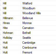
Figure 11: Simplified depiction of the index on (Surname, Location)
As we can see, there is no way for SQL Server to perform a seek operation on that index, to retrieve rows by location, since the rows are not ordered by location. Rows are ordered by surname first, and rows for a specific location are scattered through the index. Hence, if we only have a query predicate on Location and an index that has Location as a second (or third, or fourth, or…) column, then SQL Server can only use that index for a scan, not a seek.
For further coverage of this topic, see the following two blog posts:
- http://sqlinthewild.co.za/index.php/2009/01/19/index-columns-selectivity-and-equality-predicates/
- http://sqlinthewild.co.za/index.php/2009/02/06/index-columns-selectivity-and-inequality-predicates/
Query predicate is not SARGable
SARG is one of those annoying, made-up terms that tell us just about nothing. It’s an abbreviation of Search Argument and it simply means that a particular query predicate can be used for an index seek operation (which is a lovely recursive definition).
As a very high-level summary, a query predicate is SARGable if it is of the form:
|
1 |
<column name> <logical operator> <expression> |
That looks complex but, basically, it means that the column must be compared directly to an expression (function, parameter, variable or constant).
Let’s consider three example predicates:
- WHERE TransactionDate = ‘2012/01/01’
- WHERE TransactionDate > DATEADD(mm,-1,@SomeDate)
- WHERE DATEADD(dd,-1, TransactionDate) > @SomeOtherDate
Of those three, the first two are SARGable. The first example directly compares the TransactionDate column to a constant, and the second to a function.
In the third example, there is a function on the TransactionDate column; this makes the predicate non-SARGable and will result in an index scan rather than a seek (providing there’s no other SARGable predicates in the query).
To summarize, just having an index on a column is no guarantee that queries filtering on that column can use the index. The columns returned and the exact form of the predicates in the WHERE clause can both influence whether an index is useful for a query or not.
Looking for Go-faster Hints
“What hint do I add to make queries faster?”
Why not try, OPTION(GoFasterPrettyPlease)? Just kidding! There’s no hint that universally makes queries faster. Think about it, if there really were an option that made 100% of queries faster, why wouldn’t it be the default?
Many people seem to regard the NOLOCK hint (a.k.a. the Read Uncommitted isolation level), in particular, as some of “query-go-faster” switch; it is not. Rather it is an isolation level hint that allows SQL Server to ignore locks and potentially return inconsistent data (quickly). There are places and times where use of NOLOCK is tolerable, but never use it as a default hint on all queries.
If blocking is a problem, consider use of the row-versioning isolation levels, either Snapshot isolation or read committed snapshot isolation, rather than the read uncommitted isolation level, as the row-versioning isolation levels, which allow read queries to avoid use of locks and still ensure that they fetch the correct data.
The MAXDOP and RECOMPILE hints are not go-faster switches either. There are situations where they are fine, and situations where they are not (and that’s far too complex to get into in this article), but the main point is they should always be used only after careful testing.
Some hints are less “intrusive” than others and you should always try to use the least intrusive hint that achieves the desired outcome. The OPTIMIZE FOR… hints, for example, can be very useful for fixing bad parameter sniffing issues and are far less intrusive than index or join hints.
Some hints are misunderstood; for example, many people seem to think that the USE PLAN hint bypasses the optimizer, forcing use of a particular execution plan. While it’s true that the hint specifies an execution plan for the query to use, it does not bypass the optimizer and does not remove the compilation overhead. The optimizer still has to optimize (guided by the plan specified in the hint) to ensure that the plan specified is in fact a valid plan for that query. It can in some cases increase the compilation time.
In short, use hints sparingly. Reserve their use for just those times when the optimizer is not picking a desired plan, and you know exactly what the hint does, why it is used and why it is necessary, and you have tested extensively, and you are prepared to continue to test to ensure that the hint remains the best option.
Looking for Go-faster Server Configuration settings
“My server’s slow. What configuration settings do I change to make it fast?”
Again, if there were a setting that always improved query performance, it would be the default. Nevertheless, some people seem to treat certain settings as if they were a go-faster switch. The result of messing with these settings is a server with settings that differ from those generally recommended, and that may well run slower than it would with the default settings.
Personally, there are only three settings that I would generally recommend changing from their default values. Firstly, don’t leave Max server memory at the default setting, as it’s likely to result in OS memory pressure (http://www.sqlskills.com/blogs/jonathan/post/How-much-memory-does-my-SQL-Server-actually-need.aspx).
Secondly, I feel that cost threshold for parallelism is too low by default. I’ve seen recommendations to bump it to certain fixed values (I’ve seen 10, 25 and 50), but I prefer to do an analysis of the queries and pick a value tailored for the environment.
Thirdly, the value of MAXDOP may need changing from 0, but certainly not to 1, except in some specific situations, and only after extensive workload analysis has proved that this is the way to go.
Deciding the value to which it should be set is rather more complex, than just ‘use this value’. For more details on this topic, see chapter 3 of Troubleshooting SQL Server (the eBook is available as a free download), as well as Adam Machanic’s Parallelism series.
That is about it in term of settings you can and should tweak without really good reasons. Any time I do a server audit for a client I find out which server settings they have changed. If I find that settings like ‘boost priority’ or ‘lightweight pooling’ or the query memory settings (min memory per query (KB)) changed I know I’m going to find huge problems with the server because someone’s been fiddling with things best left unchanged.
In short, if you don’t know why a setting should be changed, don’t change it.
Summary
That’s just a short list, and unfortunately, I see these day after day on the forums and elsewhere. I guess the best summary would be: don’t change or implement anything without research and without knowing what it’s going to affect. Sure, that’s more work than just implementing something blindly, but it’s far more likely to achieve the desired effect.
This document contains proprietary information and is protected by copyright law.
Copyright © 2026 Red Gate Software Limited. All rights reserved
Load comments