In previous articles in this SQL Server Integration Services (SSIS) series, you’ve seen how to add a Data Flow task to your control flow and then add components to the data flow. In this article, you’ll learn how to add the Conditional Split transformation to your data flow. The transformation lets you route your data flow to different outputs, based on criteria defined within the transformation’s editor.

The example I demonstrate in this article uses the Conditional Split transformation to divide data retrieved from a table in a SQL Server database into two data flows so we can save the data into separate tables. We’ll use an OLE DB connection to retrieve the source data from the Employee table in the AdventureWorks database. We’ll then separate the data into two sets. The employees who started before 1 March 1999 will be loaded into the PreMar1999 table, and those on or after that date will be loaded into the PostMar1999 table. We’ll create these tables as we define our data flow.

Adding a Connection Manager to Our SSIS Package

Before we do anything else, we need to set up a connection manager to the database that contains our source data. To do this, right-click the Connection Manager s window and then click New OLE DB Connection, as shown in Figure 1.

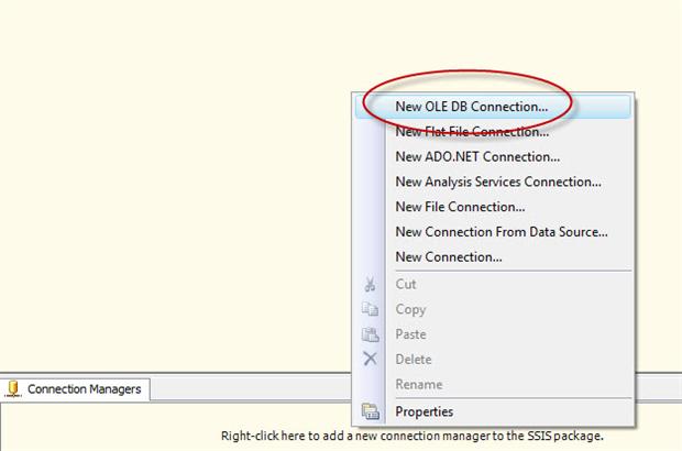
Figure 1: Adding an OLE DB connection manager

When the Configure OLE DB Connection Manager dialog box appears, click New. This launches the Connection Manager dialog box. In the Server name drop-down list, select the name of the SQL Server instance that hosts the database containing the source data you want to use for this exercise. (Note that it should be some version of the AdventureWorks database.) Then configure the authentication type you use to connect to the database. Finally, in the Connect to a database drop-down list, select the source database. On my system, I’m connecting to a SQL Server instance named 192.168.1.22/Cambridge, using SQL Server Authentication as my authentication type, and connecting to the AdventureWorks database, as shown in Figure 2.

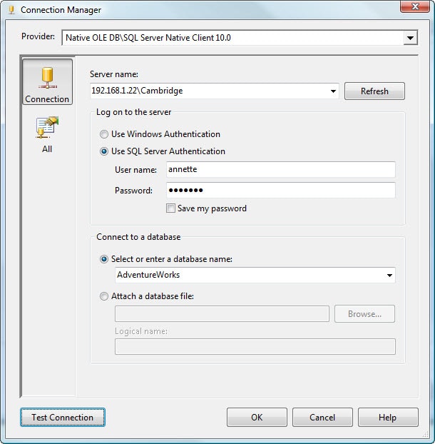
Figure 2: Configuring an OLE DB connection manager

After you set up your connection manager, click Test Connection to ensure that you can properly connect to the database. If you receive a message confirming that the test connection succeeded, click OK to close the Connection Manager dialog box. Your new connection manager should now be listed in the Connection Manager s window.

Adding an OLE DB Source to Our Data Flow

Now that we’ve established a connection to our database, we can set up our data flow to retrieve data from the Employee table and then split that data into two sets. That means we must first add a Data Flow task to our control flow. To do so, drag the task from the Control Flow Items section within the Toolbox window to the control flow design surface, as shown in Figure 3.

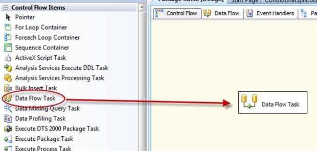
Figure 3: Adding a Data Flow task to the control flow

After you’ve added the Data Flow task, double-click the task to go to the Data Flow tab. Once there, drag an OLE DB source from the Toolbox window to the data flow design surface.

The next step is to configure the OLE DB source. To do so, double-click the component to open the OLE DB Source Editor. Because we already created an OLE DB connection manager, it will be the default value in the OLE DB connection m anager drop-down list. That’s the connection manager we want. Next, ensure that the Table or view option is selected in the Data access mode drop-down list, and then select the HumanResources.Employee table from the Name of the table or the view drop-down list. Your OLE DB Source Editor should now look similar to the one shown in Figure 4.

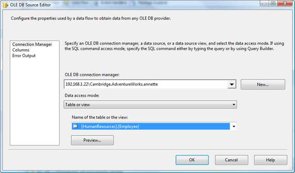
Figure 4: Configuring the OLE DB Source Editor

Now we need to select the columns we want to include in our data flow. Go to the Columns page of the OLE DB Source Editor. You’ll see a list of available columns in the Available External Columns table, as shown in Figure 5. We don’t want to include all those columns, however. We want to include only those shown in the External Column list in the grid at the bottom of the page. To remove the unwanted columns, deselect them in the Available External Columns table.

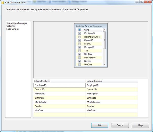
Figure 5: Selecting which columns to include in our data flow

Once your selected columns are correct, click OK to close the OLE DB Source Editor.

Adding a Conditional Split Transformation to the Data Flow

Now we need to add in the Conditional Split transformation to the data flow. To do so, drag the transformation from the Data Flow Transformations section of the Toolbox window to the data flow design surface, beneath the OLE DB source, as shown in Figure 6.

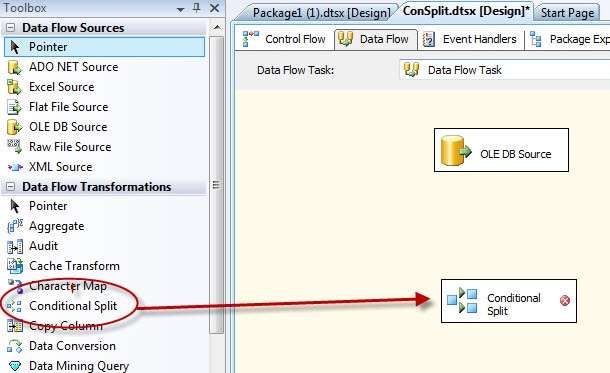
Figure 6: Adding the Conditional Split transformation to the data flow

We now need to connect the OLE DB source to the Conditional Split transformation. Click the green arrow (the data flow path) at the bottom of the OLE DB source and drag it to the Conditional Split transformation, as shown in Figure 7.

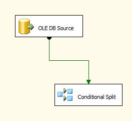
Figure 7: Connecting the source to the Conditional Split transformation

After we add the Conditional Split transformation, we need to do something with it. As I mentioned previously, we’re going to use the transformation to divide the data flow into two separate paths.

To do this, double-click on the Conditional Split transformation to open the Conditional Split Transformation Editor. The editor is divided into three main windows, as shown in Figure 8.

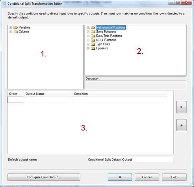
Figure 8: Working with the Conditional Split Transformation Editor

Notice in Figure 8 that I’ve labeled the windows 1, 2 and 3 to make them easier to explain. The windows provide the following functionality:

1. Columns and variables we can use in our expressions that define how to split the data flow.
2. Functions we can use in our expressions that define how to split the data flow.
3. Conditions that define how to split the data flow. These need to be set in priority order; any rows that evaluate to true for one condition will not be available to the condition that follows.

For this example, we’ll define our condition based on the HireDat e field in the data flow. So the first step to take is to expand the Columns node in window 1 and drag the HireDate field to the Condition column of the grid in window 3. When you drag the file to the Condition column, SSIS will populate the Order and Output Name columns, with all three columns written in red text as shown in Figure 9.

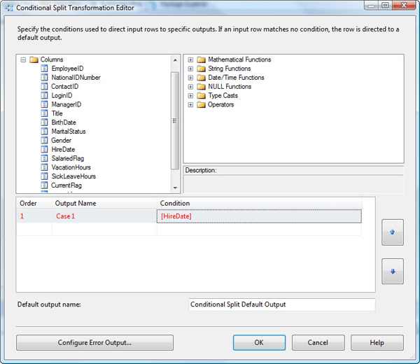
Figure 9: Creating a condition that defines how to split the data flow

As you can see in Figure 9, SSIS populates the columns with default values. For the Order column, stick with the default value of 1. For the Output Name column, we’ll provide a name for our outbound data path. (We’ll be creating two data paths, based on our split condition.) On my system, I used the name Pre Mar 1999, so type that or another name into the Output Name column. Now we must define the expression that determines how the condition will evaluate the data. This we do in the Condition column.

As previously stated, we’ll split the data flow based on those employees who started before 1 March 1999 and those who started on or after that date. So we need to define two conditions. We’ve already been working on the first condition. To finish defining that one, we need to add a comparison operator to the expression in the Condition column, in this case, the lesser-than (<) symbol. There are two ways to add the operator. You can type it directly into the Condition column (after the column name), or you can expand the Operators node in section 2 and drag the less-than symbol to the Condition column.

Next, we need to add a date for our comparison, which we add as a string literal, enclosed in double quotes. However, because we’re comparing the date to the HireDate column, we need to convert the string to the DT_DBDATE SSIS data type. Luckily, SSIS makes this very easy. We enclose the data type in parentheses and add it before the string value. Once we’ve done this, the equation in the Condition column should look as follows:

When you include the data type in this way, SSIS automatically converts the string literal to the specified data type (assuming that the string conforms to the data type’s specifications).

There are two ways you can add a data type to your equations. Either type it directly into the Condition column, or expand the Type Casts node in window 2 and drag the data type to the Condition column. Once you’ve defined your equation in the Condition column, you’re first data path is ready to go.

We now need to define our second data path. To do so, follow the same procedures as described above, only this time, use the greater-than-or-equal-to (>=) operator instead of the lesser-than one. Your second expression should be as follows:

That’s all there is to it. Your Conditional Split Transformation Editor should now look similar to the one shown in Figure 10.

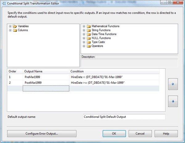
Figure 10: Setting up the Conditional Split Transformation Editor

Once you’re satisfied that you’ve configured the Conditional Split transformation the way you want it, click OK to close the Conditional Split Transformation Editor.

Adding Data Flow Destinations to the Data Flow

Now that we’ve split the data flow into multiple data paths, we now need to add a destination for each of those paths. So let’s start with the first data path. Drag an OLE DB destination from the Data Flow Destinations section of the Toolbox window to the data flow design surface, somewhere beneath the Conditional Split transformation. Next, drag the green data path arrow from the Conditional Split transformation to the OLE DB destination. When you connect the data path to the destination, the Input Output Selection dialog box appears, as shown in Figure 11. The dialog box lets us choose which output we want to direct toward the selected destination.

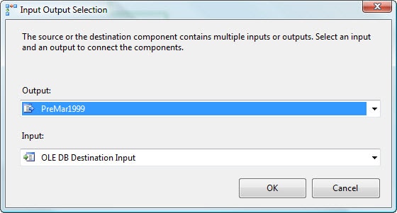
Figure 11: Configuring the Input Output Selection dialog box

Notice that the dialog box includes the Output drop-down list. These are the data path outputs available from the Conditional Split transformation. In this case, the drop-down list will include three options:

• PreMar1999
• PostMar1999
• Conditional Split Default Output

We’ve just set up the first two, so these should be self-explanatory. However, there is a third output data path, Conditional Split Default Output, which captures any records that don’t meet the conditions defined in the first two outputs. In our example, there shouldn’t be any records in this category, but later we’ll configure this one anyway, just to demonstrate how it works.

For the first OLE DB destination, select the first option, PreMar1999, and then click OK. SSIS will assign the output name to the data path. We now need to configure the OLE DB destination. Double-click the component to open the OLE DB Destination Editor. Next to the Name of the table or the view drop-down list, click the New button. This launches the Create Table dialogue box, which includes a CREATE TABLE statement that defines a table based on the data flow, as shown in Figure 12. The only change you might want to make to the statement is to modify the table name. I renamed mine to PreMar1999.

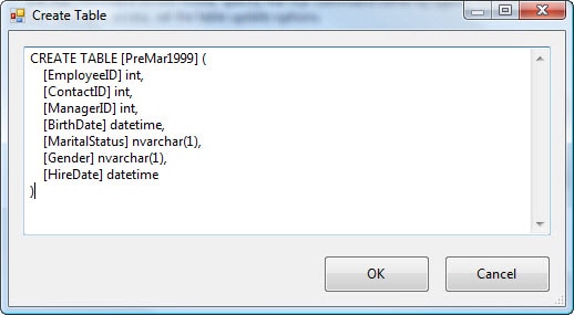
Figure 12: Creating a table when configuring the OLE DB destination

Once you’re satisfied with the CREATE TABLE statement, click OK to close the CREATE TABLE dialog box. You should be returned to the Connection Manager page of the OLE DB Destination Editor. For all other settings on this page, stick with the default values, as shown in Figure 13.

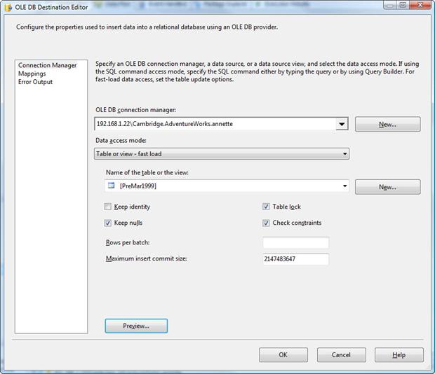
Figure 13: Using the default values in the OLE DB Destination Editor

Now go to the Mappings page of the OLE DB Destination Editor to check that the columns have mapped correctly. You can also click the Preview button on that page to ensure that the data looks as you would expect. At this stage, however, it’s likely to appear empty.

Now click OK to close the OLE DB Destination Editor.

Next, you should consider renaming your OLE DB destination to avoid confusion down the road. On my system, I renamed the destination to PreMar1999. To rename a component, right-click it, click Rename, and then type in the new name. Renaming components makes it easier to distinguish one from the other and for other developers to better understand their purpose.

Once you’ve renamed your destination, you’re ready to set up the other destinations. Repeat the data flow configuration process for the PostMar1999 data path and the default data path. You’ll notice that once a data path has been used, it’s no long available as an option.

When you’re finished configuring your OLE DB destinations and their data paths, your data flow should look similar to the one shown in Figure 14.

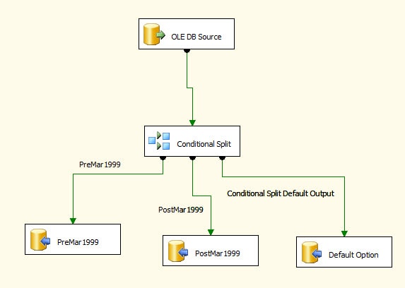
Figure 14: The data flow split into three data paths

Now it’s time to test how it works. To do this, click the Execute button (the green arrow) on the menu bar. If the package runs successfully, it should look similar to the data flow shown in Figure 15.

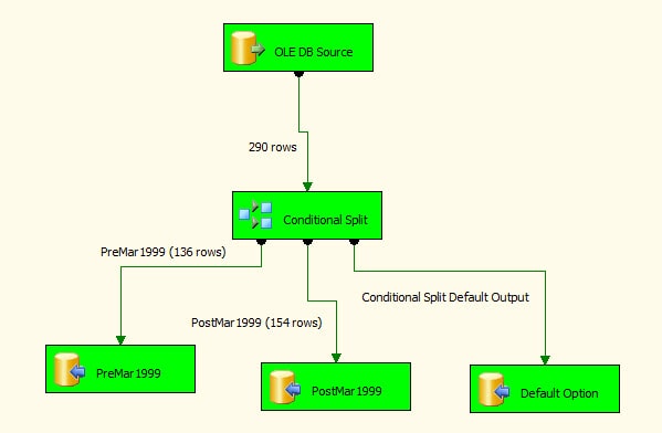
Figure 15: Running the SSIS package

If all your data flow components turn green, you know that your package is probably running correctly. However, another important indicator is the number of rows that were loaded into each table. As Figure 15 indicates, the package inserted 136 rows into the PreMar1999 table and 154 rows into the PostMar1999 table. (These numbers could vary, depending on which version of the AdventureWorks database you’re using.) As expected, no rows were passed along the default data path. If you were to check the source data (the Employee table), you should come up with a matching number of records.

Summary

In this article, we created an SSIS package with a single data flow. We added a Conditional Split transformation to the data flow in order split the data into multiple paths. We then directed each of those data paths to a different destination table. However, our destinations did not have to be SQL Server tables. They could have been flat files, spreadsheets or any other destination that SSIS supports. In future articles, we’ll use the Conditional Split with other data flow components, such as the Merge Join transformation, to insert, update and delete data.