This article is part of a three-part series on transforming and analyzing data in PostgreSQL. For more articles in this series, click here.

The first two articles in this series demonstrated how PostgreSQL is a capable tool for ELT – taking raw input and transforming it into usable data for querying and analyzing. We used sample data from the Advent of Code 2023 to demonstrate some of the ELT techniques in PostgreSQL.

In the first article, we discussed functions and features of SQL in PostgreSQL that can be used together to transform and analyze data. In the second article, we introduced Common Table Expressions (CTE) as a method to build a transformation query one step at a time to improve readability and debugging.

In this final article, I’ll tackle one last feature of SQL that allows us to process data in a loop, referencing previous iterations to perform complex calculations: Recursive CTE’s.

SQL is Set-based

SQL is primarily a set-based, declarative language. Using standard ANSII SQL and platform-specific functions, a SQL developer declares the desired outcome of a query, not the process by which the database should retrieve and process the data. The query planner typically uses statistics about the distribution of data to determine the best plan to get the desired result and return the full set of rows. While CTE’s and LATERAL joins make it feel like we can use the output of one query to impact another, those are always a one-shot opportunity. As a set-based language, it’s impossible to do algorithmic calculations, the ability to use the output of a query as input and control to another in a loop.

Stated another way, early versions of the SQL standard did not have procedural capabilities. To do that, most database platforms use their own superset of SQL that provides procedural capabilities. By default, this is T-SQL in SQL Server and pl/pgsql in PostgreSQL.

That changed with the SQL:1999 standard. With this new feature, implemented by all major databases, SQL became a Turing-complete language that can solve complex calculations in a single query.

Recursive Common Table Expressions (aka. Hierarchical Queries)

Recursive Common Table Expressions take the same form as a regular CTE. Each named query can be referred to, just like aVIEW in a later part of the query – with one major difference. Any named query can refer to back to itself in a loop, reusing the output of each iteration as input to the next until some condition is satisfied.

What does this really mean? Let’s look at a simple example.

Let’s say you wanted to return a set of data that started at number one (1) and “counted” to ten (10). In what ways might you do that using your database platform without using a recursive CTE? A few possibilities that come to mind in PostgreSQL include:

• Returning a VALUES clause with all the numbers from 1 to 10 as separate rows.
• Create a set-returning function that takes a starting and ending value as input and then uses a procedural language like pl/pgsql to loop over the data until the ending condition is met.
• Write ten different named CTE blocks, each selecting from the previous and adding 1 to the highest current value, likely with a UNION query.

Oi Vey! Notice that all these solutions are either very manual or require a superset of SQL.

Recursive CTE’s fix this.

This will return:

What just happened there? I’m glad you asked.

Recursive CTE Explained

Recursive CTE’s are straightforward to explain but often challenging to implement with real data, especially the more complex calculations you have. The example above starts with static data and builds from there. There is no table access. (we’ll get to an example of that in a bit)

To create a recursive CTE, the following rules must be satisfied:

• The keyword RECURSIVE must be added to the initial WITH keyword. This doesn’t mean the first named query in the CTE has to be recursive. Adding it indicates to the query planner that one (or more) of the named queries will refer back to itself.
• The named query must emit a set of one or more rows that is used as the starting data for the next iteration. This is referred to as the initial query.
• The second query, however complex, must reference the name of the current CTE to access the output from the previous iteration.
• A UNION/UNION ALL combines the output of the first result and each iteration thereafter.
• This process continues until a condition is met or the recursive query returns no data. Otherwise, it will perform an infinite loop and hopefully, the process will be stopped by the server to avoid crashing.

The results of each iteration are stored in a “working table” which is accessed by referencing the name of the named recursive CTE. The UNION of all the iterations is returned as the final result.

That probably feels a little abstract if you’re new to recursive CTE’s, so let’s take our first example and follow it step-by-step.

This returns:

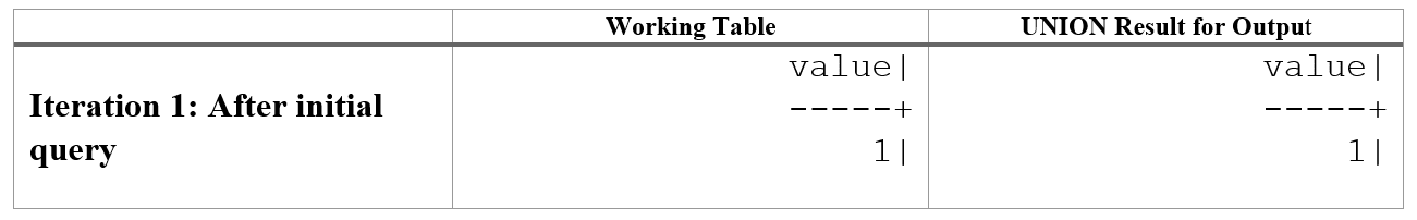
The initial query output sets the stage for the remainder of the recursive query. The hidden working table contains the output of the initial query, and the UNION output has the same data to start.

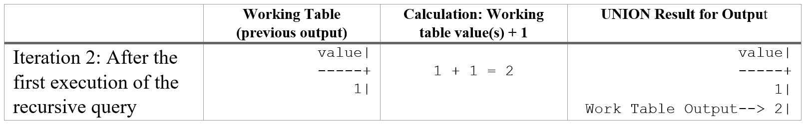
We now move to the recursive query after the UNION ALL. Because it refers back to the CTE by name (“count_value”), it can access all of the rows in the working table from the previous iteration. In our example, when the second query is executed for the first time, the working table contains one row with the “value” of 1.

As written, the query increments the ‘value’ column of all rows from the working table by one and then adds that result to the UNION output. In our case, the working table for each iteration will only have one row, so only one value will be emitted to the working table for the next iteration.

And we can keep repeating this while the value of the working table is less than 10.

.

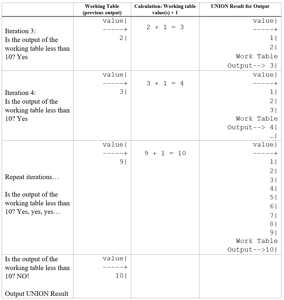
Recursive queries allow us to perform algorithmic calculations that otherwise wouldn’t be possible with standard SQL.

Hierarchical Recursive Queries

That first example didn’t select any data from a real database table. While it hopefully provided a clear, if basic, understanding of how a recursive CTE works, we need to look at a slightly more complex example.

A common use case for recursive queries is to return hierarchical data sets based on a parent/child relationship.

• Manager/Employee
• Region/Division/Territory
• Disk/Folder/Files
• Etc.

In each of these cases, the recursive query starts with an initial query that represents the top-level parent(s) and then with each iteration, selects the children for each parent. It will continue until there are no more children to select (or a certain depth of the hierarchy is reached).

To demonstrate this, let’s look at an example disk folder and file hierarchy.

The objective is to initiate the recursive query with all top-level parent folders with the initial query. The output of the initial query can then be referenced to select the first level of children folders and files. That output is stored in the working table and used during the next iteration to find any children folders or files. Rinse and repeat.

Recursive CTE Example 1

The process as it iterates through the data is as follows:

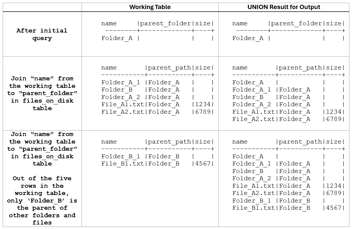
In this example, the working table sometimes had one row like the first example, but multiple rows after other iterations. The JOIN clause works like any other join. The only difference is that the contents of one table in the join (the working table) changes with each iteration.

Recursive CTE Example 2

There are a lot of ways to modify the data within a recursive CTE query to transform the final result. As long as the columns and datatypes match between the initial query and the recursive query, the sky is the limit for how the working table data is used for filtering, data modification, and more.

To demonstrate this, let’s make one small change to the query above. Notice that under the “parent_path” column the string doesn’t look like a path, just the parent folder name. However, “Folder_B” is a child of “Folder_A”. Showing that in the output would make things clearer.

This returns the following hierarchy:

Cool, huh?

Putting It All Together

Over these three articles, we’ve discussed how PostgreSQL can be used as a powerful ELT tool. We’ve shown how various functions and features likeCROSS JOIN LATERAL can be used to transform data after it’s loaded into the database. We then demonstrated how Common Table Expressions help you build a query over time and often make it more readable. Finally, we introduced and demonstrated how to use a recursive CTE in this article.

To put it all together, I’m going to use data from the Advent of Code 2022, Dec 7 puzzle.

For this puzzle, the input is a list of commands for walking through a file system. Each line either has a command like change directory (cd) or list directory (ls), or a directory name or file.

The object of the puzzle is to identify folders on the drive that can be deleted to make room for a “system update” file to fix the device. To do this, we need to identify the hierarchy of the filesystem by following the commands from beginning to end, identifying all the directories a file is a child of. Finally, the total size of files in each directory (inclusive of all children folders and files) needs to be calculated to find directories that can be deleted to create enough space for the update file to be loaded onto the device.

While that probably sounds a bit complicated, we can break up the steps using a recursive CTE and slowly build our solution.

Puzzle Input

The sample data, shown below, has 22 lines. Files are shown with the numerical size first followed by the name—directories identified after a ‘dir’ keyword.

Step 1: Identify directories and files. Everything else is noise.

This returns:

Step 2: Recursively step through the output of the first CTE, modifying the directory array as we go down or move up through the directories. Also, break out the file and size into separate columns. Note that we simply commented out the initial SELECT statement and added a second (recursive) CTE.

And this returns:

Step 3: Get a distinct set of values from the ‘dir’ column and then sum the total size of each directory, all child files included.

Returns:

Step 4: Find all directories that are less than 100,000 in total size and add them up. These are the directories that will be deleted, and we want to know how much total space will be freed.

Finally returning

Data transformation, building a query with CTE’s, and a recursive CTE to build the filesystem structure.

Conclusion

These three articles are just the tip of the iceberg for what is possible using SQL features and PostgreSQL functions. Transforming and analyzing data close to the database reduces dependencies on external tools and allows for easy modifications and updates as your process improves.

I’d recommend trying to solve puzzles from sites like the Advent of Code, and search for solutions that other SQL developers have posted to learn new tips and techniques. Each little step will improve your knowledge and hone your skills for working with data using SQL and PostgreSQL.