

The data transformation tool dbt (data build tool) has become more and more popular over the past years. It focuses heavily on SQL, and it adds a bunch of interesting features into the mix, such as data lineage, automatic orchestration, reusable macros etc. In the first article in this series, A gentle introduction to dbt, it’s explained how you can get dbt for free in the cloud version, how you can set up an account and create a connection to Microsoft Fabric. We also created our first models, where a model can eventually be persisted as a view or a table in your database. It’s recommended to go through that article first if you haven’t already, because we will build upon it.
In this article, we will dive a bit deeper into how you can specify the source tables for your dbt project, and we will create a couple of models that will load some fact and dimension tables.
How to read your Source Data
In an ELT pipeline, dbt is responsible for the “T”, meaning it can transform data that is already in the data store of choice using SQL. This means that some other tool – this can be pipelines in Azure Data Factory or in Fabric – needs to be responsible for extracting source data and storing it in your database. Suppose this part of the process has already been completed and you have data available for you in staging tables. How can you process that data with dbt?
Get sample data in Fabric SQL DB
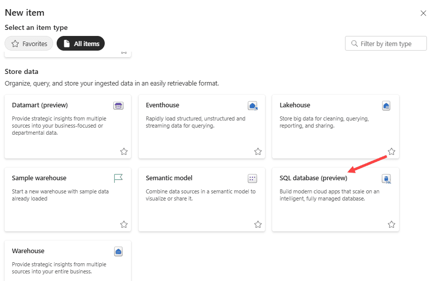
As a source, we’ll use sample data loaded into a SQL DB in Microsoft Fabric (this feature is in preview since the Microsoft Ignite 2024 conference). In a Fabric-enabled workspace, you can find the SQL database item under the “store data” category when you want to add a new item.
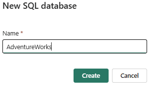
Give the new database a name. This name will be displayed when you connect to the database with the SQL Analytics Endpoint (which reads the mirrored Parquet files in the delta lake storage).
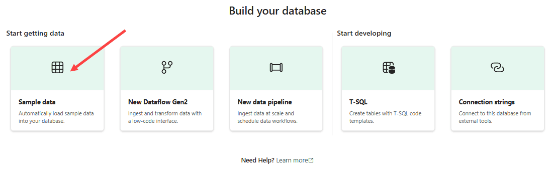
Once the database is provisioned, you’re presented with multiple options to load data into it. In our case, we want to load the sample AdventureWorksLT database.
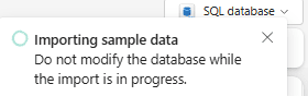
It might take a little while to load the data.
When the database is ready, you can see several tables are loaded into the SalesLT schema:
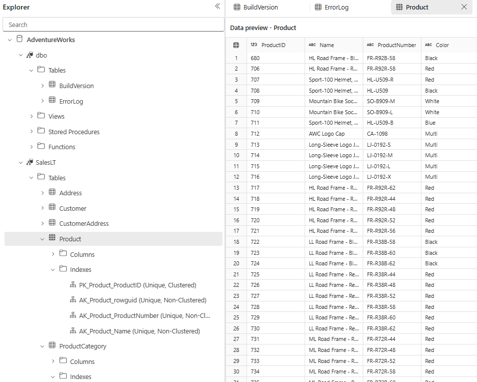
We will now try to read and transform this data in dbt.
Specifying the Sources in dbt
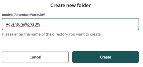
dbt needs to know where it can find the source tables. The declaration of the source tables is done in a YAML file. Let us first add a new folder to the dbt project and
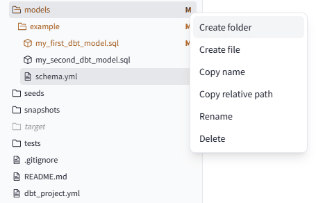
Name it “AdventureWorksDW”:
Using the same context menu, we can add a new YAML file to this folder:
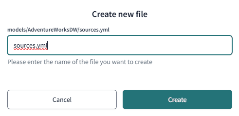
The file doesn’t necessarily need to be called sources.yml, but inside the YAML file there needs to be a sources: key in the file. In the file, we place the following contents:
|
1 2 3 4 5 6 7 8 9 10 11 |
version: 2 sources: - name: adventureworkslt database: AdventureWorks schema: SalesLT tables: - name: Product - name: ProductCategory - name: ProductDescription - name: ProductModel - name: ProductModelProductDescription |
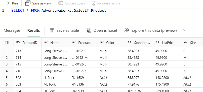
We gave our source a name – adventureworkslt – and we specify the name of the database, the schema and the names of the different tables. Because the warehouse can use three-part naming, we can access the tables in the SQL DB from the warehouse itself. This uses the SQL Analytics Endpoint of the SQL DB. For example:
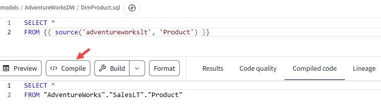
In the folder we created earlier, we can now add a new file called DimProduct.sql. It’s important to include the .sql extension, so dbt can recognize it as a model. Inside the file, we can add the following SQL, which includes a jinja reference to one of the source tables we specified in the sources.yml file:
|
1 2 |
SELECT * FROM {{ source('adventureworkslt', 'Product') }} |
The reference consists of the source name and the name of the table. At compile time, dbt will translate this to the correct three-part name:
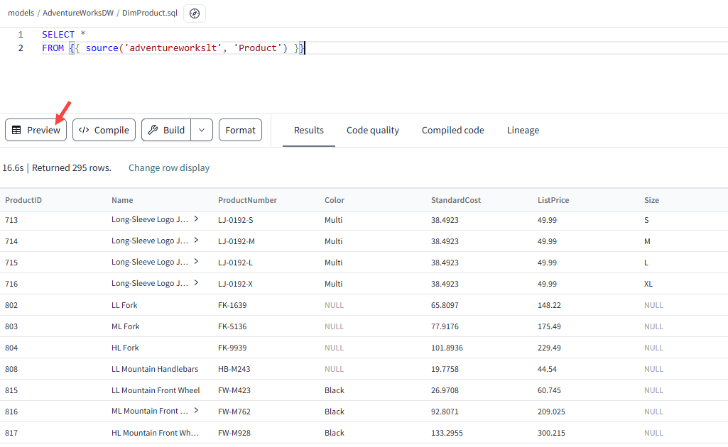
It’s also possible to do a preview of the data, if the SQL statement is valid:
Let’s change our query with something more complex; we now read from several source tables in the same query:
|
1 2 3 4 5 6 7 8 9 10 11 12 13 14 15 16 17 18 19 20 21 22 23 24 25 26 27 28 29 30 31 32 33 34 35 36 37 38 39 40 41 42 43 44 45 46 47 48 49 |
WITH cte_categories AS ( SELECT ProductCategoryID ,ProductCategoryName = [Name] FROM {{ source('adventureworkslt', 'ProductCategory') }} WHERE ParentProductCategoryID IS NULL ) , cte_subcategories AS ( SELECT ProductSubCategoryID = sc.ProductCategoryID ,ProductSubCategoryName = sc.[Name] ,c.ProductCategoryName FROM {{ source('adventureworkslt', 'ProductCategory') }} sc LEFT JOIN cte_categories c ON sc.ParentProductCategoryID = c.ProductCategoryID WHERE ParentProductCategoryID IS NOT NULL ) , cte_models AS ( SELECT m.ProductModelID ,ProductModelName = m.[Name] ,ProductModelDesc = ISNULL(d.[Description],'Description missing...') FROM {{ source('adventureworkslt', 'ProductModel') }} m LEFT JOIN {{ source('adventureworkslt', 'ProductModelProductDescription') }} md ON m.ProductModelID = md.ProductModelID AND md.Culture = 'en' LEFT JOIN {{ source('adventureworkslt', 'ProductDescription') }} d ON md.ProductDescriptionID = d.ProductDescriptionID ) SELECT p.ProductID ,ProductName = p.[Name] ,p.ProductNumber ,ProductColor = ISNULL(p.Color,'N/A') ,p.StandardCost ,p.ListPrice ,ProductSize = ISNULL(p.Size,'N/A') ,ProductWeight = p.[Weight] ,p.SellStartDate ,p.SellEndDate ,p.DiscontinuedDate ,ProductSubCategoryName = ISNULL(pc.ProductSubCategoryName,'N/A') ,ProductCategoryName = ISNULL(pc.ProductCategoryName,'N/A') ,ProductModelName = ISNULL(m.ProductModelName,'N/A') ,ProductModelDesc = ISNULL(m.ProductModelDesc,'N/A') FROM {{ source('adventureworkslt', 'Product') }} p LEFT JOIN cte_subcategories pc ON p.ProductCategoryID = pc.ProductSubCategoryID LEFT JOIN cte_models m ON p.ProductModelID = m.ProductModelID; |
When we save and compile the model, we get an updated lineage view, which shows the dependencies of the model on the source tables:
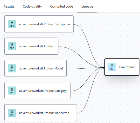
This only works if you use the source macro to reference the source tables, if you would hardcode the table names the lineage view will not show the dependencies. We can now create a similar model for the customers. First, we will need to append the names of the source tables to the sources.yml file:
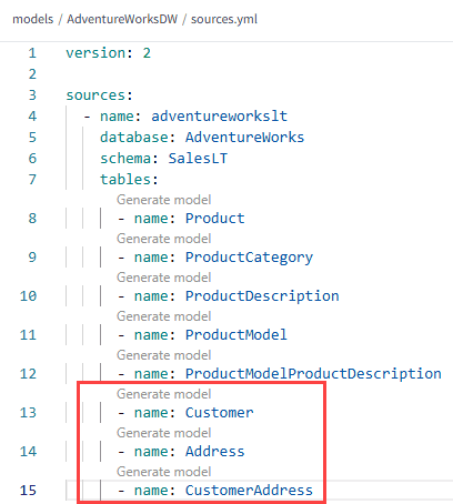
Add a new file called DimCustomer.sql and add the following SQL statement:
|
1 2 3 4 5 6 7 8 9 10 11 12 13 14 15 16 17 18 19 20 21 22 23 24 25 26 27 |
WITH cte_mainoffices AS ( SELECT ca.CustomerID ,a.City ,a.StateProvince ,a.CountryRegion ,a.PostalCode FROM {{ source('adventureworkslt', 'CustomerAddress') }} ca JOIN {{ source('adventureworkslt', 'Address') }} a ON ca.AddressID = a.AddressID WHERE ca.AddressType = 'Main Office' ) SELECT c.CustomerID ,CustomerName = CONCAT_WS(' ',c.Title, c.FirstName, c.MiddleName, c.LastName, c.Suffix) ,CustomerCompanyName = ISNULL(c.CompanyName,'N/A') ,CustomerSalesPerson = ISNULL(c.SalesPerson,'N/A') ,CustomerEmail = ISNULL(c.EmailAddress,'N/A') ,CustomerPhone = ISNULL(c.Phone,'N/A') ,CustomerPostalCode = ISNULL(m.PostalCode,'N/A') ,CustomerCity = ISNULL(m.City,'N/A') ,CustomerStateProvince = ISNULL(m.StateProvince,'N/A') ,CustomerCountryRegion = ISNULL(m.CountryRegion,'N/A') FROM {{ source('adventureworkslt', 'Customer') }} c LEFT JOIN cte_mainoffices m ON c.CustomerID = m.CustomerID; |
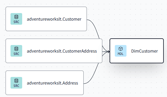
Resulting in this lineage view:
For our final model, FactSales.sql, we can use the following SQL statement (don’t forget to add the two extra source tables to the sources.yml file!).
|
1 2 3 4 5 6 7 8 9 10 11 12 13 14 15 16 17 18 19 20 21 22 23 24 25 26 27 28 29 30 31 32 33 34 35 36 37 38 39 40 41 42 43 44 45 46 47 48 49 50 51 52 |
WITH cte_details AS ( SELECT SalesOrderID ,SalesOrderDetailID ,OrderQty ,ProductID ,UnitPrice ,UnitPriceDiscount ,LineTotal = ISNULL(OrderQty * (1.0 - ISNULL(UnitPriceDiscount,0.0)) * UnitPrice,0.0) FROM {{ source('adventureworkslt', 'SalesOrderDetail') }} ), cte_sales AS ( SELECT soh.SalesOrderID ,sod.SalesOrderDetailID ,SK_OrderDate = CONVERT(DATE,soh.OrderDate) ,SK_DueDate = CONVERT(DATE,soh.DueDate) ,SK_ShipDate = CONVERT(DATE,soh.ShipDate) ,soh.PurchaseOrderNumber ,soh.AccountNumber ,soh.CustomerID ,sod.ProductID ,sod.OrderQty ,sod.UnitPrice ,sod.UnitPriceDiscount ,sod.LineTotal /* the next two costs are evenly divided over the detail lines */ ,TaxAmt = soh.TaxAmt / (COUNT(1) OVER (PARTITION BY soh.SalesOrderID)) ,Freight = soh.Freight / (COUNT(1) OVER (PARTITION BY soh.SalesOrderID)) FROM {{ source('adventureworkslt', 'SalesOrderHeader') }} soh JOIN cte_details sod ON soh.SalesOrderID = sod.SalesOrderID ) SELECT SalesOrderID ,SalesOrderDetailID ,SK_OrderDate ,SK_DueDate ,SK_ShipDate ,PurchaseOrderNumber ,AccountNumber ,CustomerID ,ProductID ,OrderQty ,UnitPrice ,UnitPriceDiscount ,LineTotal ,TaxAmt ,Freight ,TotalAmount = LineTotal + ISNULL(TaxAmt,0.0) + ISNULL(Freight,0.0) FROM cte_sales; |
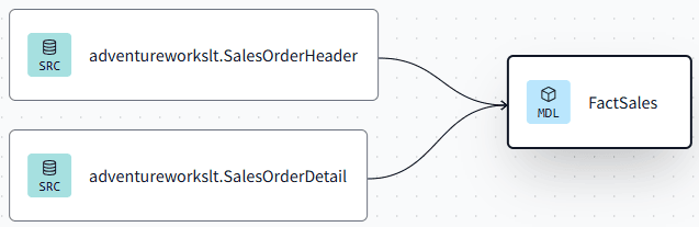
Which will result in this lineage view:
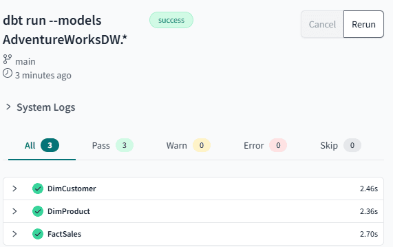
Our (simple) data warehouse is finished, for now. We can build all the models and deploy them to the Fabric warehouse with the following command:
|
1 |
dbt run --models AdventureWorksDW.* |
This command will take all compiled models within the path specified and execute them against the database.
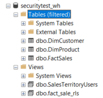
However, the models are created as views, not as tables.
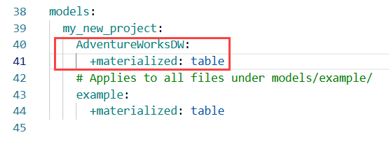
This is the default in dbt, but we can override this by setting it in the model itself. If you want to do this for an entire folder, you can specify the behaviour in the dbt_project.yml file.
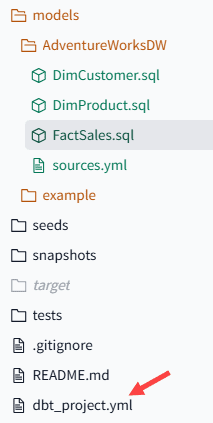
Add the folder and the +materialized keyword and set it to Table:
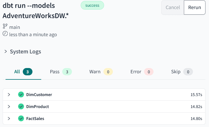
When we run the command again, we can see load times have increased as data is loaded into tables:
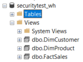
The views have been removed and tables have been created instead:
Conclusion
In this article, we showed how you can load sample data into a Fabric SQL Database. Then we used this data to load a couple of models in dbt. We needed to specify those source tables in a YAML file, which allows metadata references inside the SQL statement, allowing dbt to derive dependencies and create a lineage view.
Those models aren’t “best practice” yet when it comes to data warehouse modelling. In a following article, we will discover how we can use macros to add surrogate keys, reuse code and create a date dimension.
This document contains proprietary information and is protected by copyright law.
Copyright © 2026 Red Gate Software Limited. All rights reserved


Load comments