
Data Lakes are becoming more usual every day and the need for tools to query them also increases.
While writing about querying a data lake using Synapse, I stumbled upon a Power BI feature I didn’t know was there.
When reading from a data lake, each folder is like a table. We store in the folder many files with the same structure, each file containing a piece of the data.
Data Lake tools are prepared to deal with the data on this way and read the files transparently for the user, but Power BI required us to read one specific file, not the folder. That’s until last November. If we google (verb: To google) about Power BI and Parquet files we can find many work arounds to read Parquet files in Power BI, but no mention to the new Parquet connector released on last November (https://powerbi.microsoft.com/en-us/blog/whats-new-in-power-query-dataflows-november-2020/), so I had to write about it.
The feature I’m illustrating on this article is in fact a combination of two features:
- The feature to combine multiple files from Azure Data Lake Gen 2 storage. This was in preview in October 2019 in is available for a while, but I was surprised I couldn’t find any article really explaining the M code used to combine the files and how to customize the code.
- The Parquet connector is the responsible to read Parquet files and adds this feature to the Azure Data Lake Gen 2. This connector was released in November 2020.
In order to illustrate how it works, I provided some files to be used in an Azure Storage. You can download the files here. You will also need to provision a new storage account and it will need to be an Azure Data Lake Storage Gen 2.
On the examples, I will use the address https://lakedemo.dfs.core.windows.net/opendatalake/trips for the storage, but you need to replace it with the DFS endpoint of your own storage.
Let’s make a step-by step:
- Open Power BI
- Select Get Data option on the main screen
- Select Azure Data Lake Storage Gen2. We will test directly with one of the most efficient options
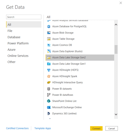
There are 3 storage options:
- Azure Blob Storage
- Data Lake Storage Gen 1
- Azure Data Lake Storage Gen 2
It’s important to choose the correct option according your storage type, this affects the performance.
- On the URL box, type this URL: https://lakedemo.dfs.core.windows.net/opendatalake/trips
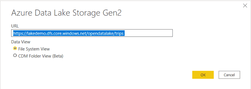
- Click Ok button
- Click the Combine button
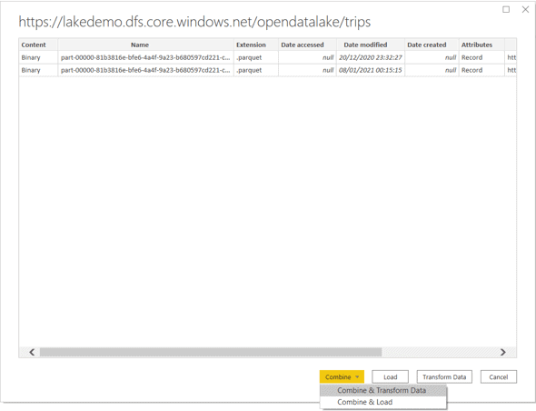
This screen has the traditional Transform and Load buttons but also has the Combine button, which has both options, Transform and Load, below it.
The traditional Transform and Load will be dealing with the list of files inside the Azure Storage folder. From this point, it will be our decision what to do with each file.
The Combine button, on the other hand, will bring to us a pre-built M script to combine all the files in the folder. It’s easy to mistake this feature believing Power BI will read only the current files, but in fact the script is flexible in such a way to read all the files in the folder, even future files included there.
- Select the option Combine & Transform
- Click Transform Data button
The M Code – How it Works
On Power Query window, you may notice the pre-built steps in the Applied Steps window. It’s also very interesting the way the queries were built: The final query is in a folder called Other Queries while you also have a folder called Helper Function containing a parameterized function.
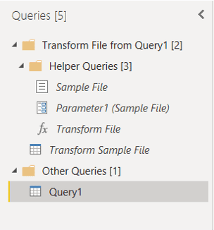
Let’s analyze the M code to better understand how it works. Using the menu View-> Advanced Editor you can access the M code.
This is how our M code looks like:
Source = AzureStorage.DataLake(“https://lakedemo.dfs.core.windows.net/opendatalake/trips”),
#”Filtered Hidden Files1″ = Table.SelectRows(Source, each [Attributes]?[Hidden]? <> true),
#”Invoke Custom Function1″ = Table.AddColumn(
#”Filtered Hidden Files1″,
“Transform File”,
each #”Transform File”([Content])
),
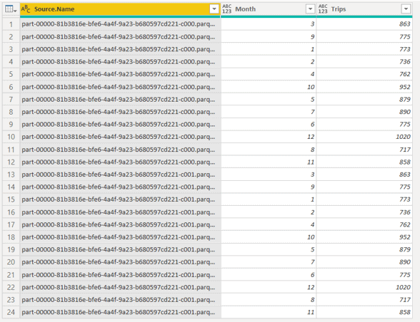
#”Renamed Columns1″ = Table.RenameColumns(#”Invoke Custom Function1″, {“Name”, “Source.Name”}),
#”Removed Other Columns1″ = Table.SelectColumns(
#”Renamed Columns1″,
{“Source.Name”, “Transform File”}
),
#”Expanded Table Column1″ = Table.ExpandTableColumn(
#”Removed Other Columns1″,
“Transform File”,
Table.ColumnNames(#”Transform File”(#”Sample File”))
),
#”Removed Columns” = Table.RemoveColumns(#”Expanded Table Column1″, {“Source.Name”}),
#”Grouped Rows” = Table.Group(
#”Removed Columns”,
{“Month”},
{{“Trips”, each List.Sum([Trips]), type number}}
)
in
#”Grouped Rows”
These are the steps this code is executing:
- Filter all files, making sure to not include hidden files
- Use the AddColumn method to call the function “Transform File” for each row
- Remove additional columns, leaving only the file name and result of the function
- Expands the column containing the result of the function
This main script calls the Transform File function for each file in the folder. There is no fixed file name, all the files will be transformed and returned. This means that at any time new files are included in this data lake folder, a simple refresh will bring the data to the dashboard, leaving the solution flexible as a client solution for a data lake needs to be.
The M code for the Transform File function is this:
Source = Parquet.Document(Parameter1),
#”Changed Type” = Table.TransformColumnTypes(Source,{{“DateID”, type text}}),
#”Added Custom” = Table.AddColumn(#”Changed Type”, “Month”, each Text.Middle([DateID],4,2)),
#”Grouped Rows” = Table.Group(#”Added Custom”, {“Month”}, {{“Trips”, each Table.RowCount(_), Int64.Type}}),
#”Changed Type1″ = Table.TransformColumnTypes(#”Grouped Rows”,{{“Month”, Int64.Type}})
in
#”Changed Type1″
The function is using the Parquet connector released in November to process the file.
Additional Transformations
Probably we would like to make additional transformations to the data. For that, we have a choice to make: If we make the transformations on the main query, all the files will be combined first and only after the combine our transformations will be executed.
On the other hand, we have the option to make the transformations inside the function. If we do so, the transformations will be applied for each file before combining them. When they are combined, they will already be with the transformed result set.
For each transformation, we will need to identify if it will perform better when executed for each file or when executed over the combined result.
Let’s compare both options.
Transformations on the Combined Result
- Select the main query, Query1
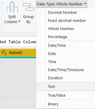
- Select the DateID column
- On the top bar, change Data Type to Text
- Click the Add Column menu
- Click Custom Column button
- On New Column Name box, set the name as Month
- On Custom Column Formula box, set the expression as =Text.Middle([DateID],4,2)
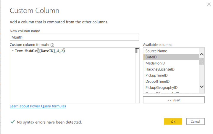
- Click Ok
- Click the Group By button
- Select the Month column
- On New Column Name box type Trips
- Keep the default Operation, Count Rows
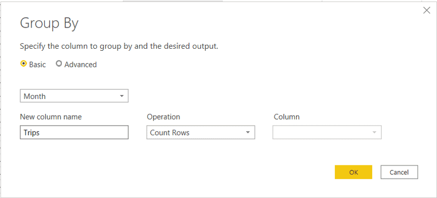
- Click Ok
- Select the Month column
- On the top bar, change Data Type to Whole Number
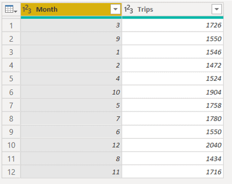
That’s it, our ETL is ready to be used on the dashboards. Let’s check the execution time of the ETLs
- Click Tools menu
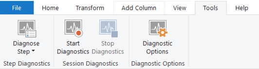
- Click the Start Diagnostics button
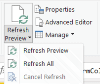
- Click Home menu
- Open the Refresh Preview drop down
- Click Refresh All menu item
- Click Tools menu
- Click Stop Diagnostics button
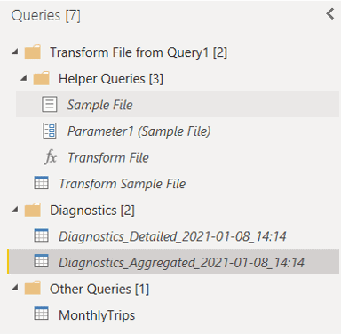
On the left side of the screen, in the query window, you will find a new folder called Diagnostics with two queries inside the folder, holding the results of the diagnostics.
- Click the Diagnostics_Aggregate query
- On the StartTime column header, open the drop down
- Click the Sort Ascending menu item
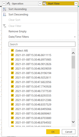
- Take note of the time on the first record
- On the StartTime column header, open the drop down
- Click Clear Sort menu item
- On the EndTime column header, open the drop down menu
- Click the Sort Descending menu item
- Take note of the time on the first record
- Calculate the time difference between the first time and the 2nd time you took note
In my example, the total time was 7 seconds. You may find slight differences.
Transformations on Each File
Let’s build the example again, this time building the transformations inside the function, so they would be applied for each file instead of the final result.
- Repeat the steps 1-7 from previous steps again
- Select the Transform Sample File query
- With the Transform Sample File query selected, repeat the steps 9-23
- Select the main query, Query1
- Remove the last step in Applied Steps window, the Change Type step
- Select the first column, Source.Name
- Click the Remove Column button
- Click Group By button
- Select the Month column
- In the New Column Name box, type Month
- On Operation drop down, select Sum
- On Column drop down, select Trips
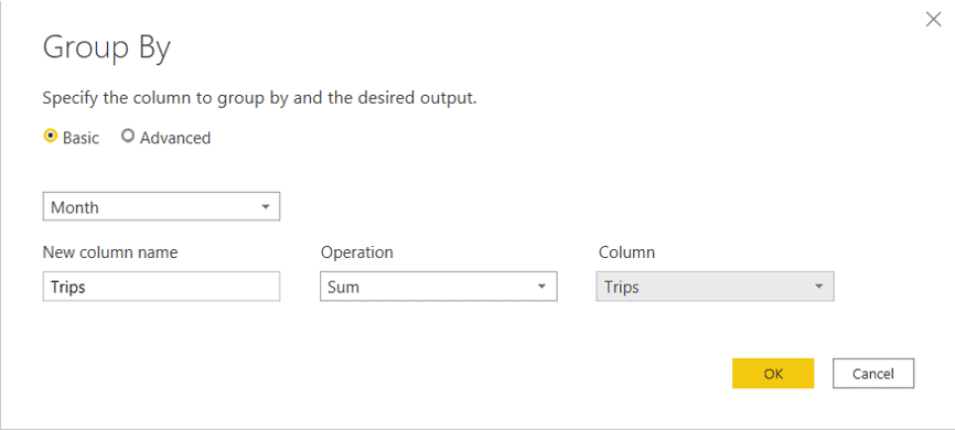
- Click Ok
- Repeat Steps 24-39
On my example, the execution time results in 4 seconds.
Conclusion
As you may notice, on this example the transformations made on each file performed better than the transformations made after the final combination. This illustrates how important it is to understand this structure and test the performance, deciding which one will perform better for your transformations.
This new feature may not be so obvious, hidden in a Combine button and a complex M code structure, but it’s still much better than possible work arounds for the problem.
This document contains proprietary information and is protected by copyright law.
Copyright © 2026 Red Gate Software Limited. All rights reserved


Load comments