
The SQL Server Query Optimizer is a cost-based optimizer. It analyzes a number of candidate execution plans for a given query, estimates the cost of each of these plans and selects the plan with the lowest cost of the choices considered. Indeed, given that the Query Optimizer cannot consider every possible plan for every query, it actually has to do a cost-based balancing act, considering both the cost of finding potential plans and the costs of plans themselves.
Therefore, it is the SQL Server component that has the biggest impact on the performance of your databases. After all, selecting the right (or wrong) execution plan could mean the difference between a query execution time of milliseconds, and one of minutes or even hours. Naturally, a better understanding of how the Query Optimizer works can help both database administrators and developers to write better queries and to provide the Query Optimizer with the information it needs to produce efficient execution plans.
This article starts with an overview on how the SQL Server Query Optimizer works and introduces the concepts that I cover in more detail in my book. We’ll also cover some of the background and challenges of query optimization, such as cardinality and cost estimations, and a section on how to read and understand them is included as well. We’ll end with a discussion of join ordering, one of the most complex problems in query optimization, and shows how joining tables in an efficient order improves the performance of a query but, at the same time, can exponentially increase the number of execution plans that should be analyzed by the Query Optimizer.
Note: This article contains a large number of example SQL queries, all of which are based on the AdventureWorks database. All code has been tested for these databases on both SQL Server 2008 and SQL Server 2008 R2. Note that these sample databases are not included in your SQL Server installation by default, but can be downloaded from the CodePlex web site. You need to download the family of sample databases for your version, either SQL Server 2008 or SQL Server 2008 R2. During installation you may choose to install all the databases or at least the AdventureWorks and AdventureWorksDW.
How the Query Optimizer Works
At the core of the SQL Server Database Engine are two major components: the Storage Engine and the Query Processor, also called the Relational Engine. The Storage Engine is responsible for reading data between the disk and memory in a manner that optimizes concurrency while maintaining data integrity. The Query Processor, as the name suggests, accepts all queries submitted to SQL Server, devises a plan for their optimal execution, and then executes the plan and delivers the required results.
Queries are submitted to SQL Server using the SQL language (or T-SQL, the Microsoft SQL Server extension to SQL). Since SQL is a high-level declarative language, it only defines what data to get from the database, not the steps required to retrieve that data, or any of the algorithms for processing the request. Thus, for each query it receives, the first job of the query processor is to devise a plan, as quickly as possible, which describes the best possible way to execute said query (or, at the very least, an efficient way). Its second job is to execute the query according to that plan.
Each of these tasks is delegated to a separate component within the query processor; the Query Optimizer devises the plan and then passes it along to the Execution Engine, which will actually execute the plan and get the results from the database.
In order to arrive at what it believes to be the best plan for executing a query, the Query Processor performs a number of different steps; the entire query processing process is shown on figure 1-1.
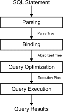
Figure 1 – The Query Processing Process
- Parsing and binding – the query is parsed and bound. Assuming the query is valid, the output of this phase is a logical tree, with each node in the tree representing a logical operation that the query must perform, such as reading a particular table, or performing an inner join. This logical tree is then used to run the query optimization process, which roughly consists of the following two steps;
- Generate possible execution plans – using the logical tree, the Query Optimizer devises a number of possible ways to execute the query i.e. a number of possible execution plans. An execution plan is, in essence, a set of physical operations (an index seek, a nested loop join, and so on), that can be performed to produce the required result, as described by the logical tree;
- Cost-assessment of each plan – While the Query Optimizer does not generate every possible execution plan, it assesses the resource and time cost of each plan it does generate. The plan that the Query Optimizer deems to have the lowest cost of those it’s assessed is selected, and passed along to the Execution Engine;
- Query execution, plan caching – the query is executed by the Execution Engine, according to the selected plan. The plan may be stored in memory, in the plan cache.
Parsing and binding are the first operations performed when a query is submitted to a SQL Server instance. Parsing makes sure that the T-SQL query has a valid syntax, and translates the SQL query into an initial tree representation: specifically, a tree of logical operators representing the high-level steps required to execute the query in question. Initially, these logical operators will be closely related to the original syntax of the query, and will include such logical operations as “get data from the Customer table”, “get data from the Contact table”, “perform an inner join”, and so on. Different tree representations of the query will be used throughout the optimization process, and this logical tree will receive different names until it is finally used to initialize the Memo structure, as will be discussed later.
Binding is mostly concerned with name resolution. During the binding operation, SQL Server makes sure that all the object names do exist, and associates every table and column name on the parse tree with their corresponding object in the system catalog. The output of this second process is called an algebrized tree, which is then sent to the Query Optimizer.
The next step is the optimization process, which is basically the generation of candidate execution plans and the selection of the best of these plans according to their cost. As has already been mentioned, SQL Server uses a cost-based optimizer, and uses a cost estimation model to estimate the cost of each of the candidate plans.
In essence, query optimization is the process of mapping the logical query operations expressed in the tree representation to physical operations, which can be carried out by the execution engine. So it’s actually the functionality of the execution engine that is being implemented in the execution plans being created by the Query Optimizer, that is, the execution engine implements a certain number of different algorithms and it is from these algorithms that the Query Optimizer must choose, when formulating its execution plans. It does this by translating the original logical operations into the physical operations that the execution engine is capable of performing, and execution plans show both the logical and physical operations. Some logical operations, such as a Sort, translate to the same physical operation, whereas other logical operations map to several possible physical operations. For example, a logical join can be mapped to a Nested Loops Join, Merge Join, or Hash Join physical operator.
Thus, the end product of the query optimization process is an execution plan: a tree consisting of a number of physical operators, which contain the algorithms to be performed by the execution engine in order to obtain the desired results from the database.
Generating Candidate Execution Plans
As discussed, the basic purpose of the Query Optimizer is to find an efficient execution plan for your query. Even for relatively simple queries, there may be a large number of different ways to access the data to produce the same end result. As such, the Query Optimizer has to select the best possible plan from what may be a very large number of candidate execution plans, and it’s important that it makes a wise choice, as the time it takes to return the results to the user can vary wildly, depending on which plan is selected.
The job of the Query Optimizer is to create and assess as many candidate execution plans as possible, within certain criteria, in order to arrive at the best possible plan. We define the search space for a given query as the set of all the possible execution plans for that query, and any possible plan in this search space returns the same results. Theoretically, in order to find the optimum execution plan for a query, a cost-based query optimizer should generate all possible execution plans that exist in that search space and correctly estimate the cost of each plan. However, some complex queries may have thousands or even millions of possible execution plans and, while the SQL Server Query Optimizer can typically consider a large number of candidate execution plans, it cannot perform an exhaustive search of all the possible plans for every query. If it did, then the time taken to assess all of the plans would be unacceptably long, and could start to have a major impact on the overall query execution time.
The Query Optimizer must strike a balance between optimization time and plan quality. For example, if the Query Optimizer spends one second finding a good enough plan that executes in one minute, then it doesn’t make sense to try to find the perfect or most optimal plan, if this is going to take five minutes of optimization time, plus the execution time. So SQL Server does not do an exhaustive search, but instead tries to find a suitably efficient plan as quickly as possible. As the Query Optimizer is working within a time constraint, there’s a chance that the plan selected may be the optimal plan but it is also likely that it may just be something close to the optimal plan.
In order to explore the search space, the Query Optimizer uses transformation rules and heuristics. The generation of candidate execution plans is performed inside the Query Optimizer using transformation rules, and the use of heuristics limits the number of choices considered in order to keep the optimization time reasonable. Candidate plans are stored in memory during the optimization, in a component called the Memo.
Assessing the Cost of each Plan
Searching, or enumerating candidate plans is just one part of the optimization process. The Query Optimizer still needs to estimate the cost of these plans and select the least expensive one. To estimate the cost of a plan, it estimates the cost of each physical operator in that plan using costing formulas that consider the use of resources such as I/O, CPU, and memory. This cost estimation depends mostly on the algorithm used by the physical operator, as well as the estimated number of records that will need to be processed; this estimate of the number of records is known as the cardinality estimation.
To help with this cardinality estimation, SQL Server uses and maintains optimizer statistics, which contain statistical information describing the distribution of values in one or more columns of a table. Once the cost for each operator is estimated using estimations of cardinality and resource demands, the Query Optimizer will add up all of these costs to estimate the cost for the entire plan.
Query Execution and Plan Caching
Once the query is optimized, the resulting plan is used by the Execution Engine to retrieve the desired data. The generated execution plan may be stored in memory, in the plan cache (known as the procedure cache in previous versions of SQL Server) in order that it might be reused if the same query is executed again. If a valid plan is available in the plan cache, then the optimization process can be skipped and the associated cost of this step, in terms of optimization time, CPU resources, and so on, can be avoided.
However, reuse of an existing plan may not always be the best solution for a given query. Depending on the distribution of data within a table, the optimal execution plan for a given query may differ greatly depending on the parameters provided in said query, and a behavior known as parameter sniffing may result in a suboptimal plan being chosen.
Even when an execution plan is available in the plan cache, some metadata changes, such as removing an index or a constraint, or significant enough changes made to the contents of the database, may render an existing plan invalid or suboptimal, and thus cause it to be discarded from the plan cache and a new optimization to be generated. As a trivial example, removing an index will make a plan invalid if the index is used by that plan. Likewise, the creation of a new index could make a plan suboptimal, if this index could be used to create a more efficient alternative plan, and enough changes to the database contents may trigger an automatic update of statistics, with the same effect on the existing plan.
Plans may also be removed from the plan cache when SQL Server is under memory pressure or when certain statements are executed. Changing some configuration options, for example max degree of parallelism, will clear the entire plan cache. Alternatively, some statements, like altering a database with certain ALTER DATABASE options will clear all the plans associated with that particular database.
Hinting
Most of the time, the Query Optimizer does a great job at choosing highly efficient execution plans. However, there may be cases when the selected execution plan does not perform as expected. It is vitally important to differentiate between when these cases arise because you are not providing the Query Optimizer with all the information it needs to do a good job, and when the problem arises because of a Query Optimizer limitation.
The reality is that, even after more than 30 years of research, query optimizers are highly complex pieces of software which still face some technical challenges, some of which will be mentioned in the next section. As a result, there may be cases when, even after you’ve provided the Query Optimizer with all the information it needs and there doesn’t seem to be any apparent problem, you are still not getting an efficient plan; in these cases you may want to resort to hints. However, since hints let you to override the operations of the Query Optimizer, they need to be used with caution, and only as a last resort when no other option is available. Hints are instructions that you can send to the Query Optimizer to influence a particular area of an execution plan. For example, you can use hints to direct the Query Optimizer to use a particular index or a specific join algorithm. You can even ask the Query Optimizer to use a specific execution plan, provided that you specify one in XML format.
Ongoing Query Optimizer Challenges
Query optimization is an inherently complex problem, not only in SQL Server but in any other relational database system. Despite the fact that query optimization research dates back to the early seventies, challenges in some fundamental areas are still being addressed today. The first major impediment to a query optimizer finding an optimal plan is the fact that, for many queries, it is just not possible to explore the entire search space. An effect known as combinatorial explosion makes this exhaustive enumeration impossible, as the number of possible plans grows very rapidly depending on the number of tables joined in the query. To make the search a manageable process, heuristics are used to limit the search space. However, if a query optimizer is not able to explore the entire search space, there is no way to prove that you can get an absolutely optimal plan, or even that the best plan is among the candidate being considered. As a result, it is clearly extremely important that the set of plans which a query optimizer considers contains plans with low costs.
This leads us to another major technical challenge for the Query Optimizer: accurate cost and cardinality estimation. Since a cost-based optimizer selects the execution plan with the lowest cost, the quality of the plan selection is only as good as the accuracy of the optimizer’s cost and cardinality estimations. Even supposing that time is not a concern and that the query optimizer can analyze the entire search space without a problem, cardinality and cost estimation errors can still make a a query optimizer select the wrong plan. Cost estimation models are inherently inexact, as they do not consider all of the hardware conditions, and must necessarily make certain assumptions about the environment. For example, the costing model assumes that every query starts with a cold cache; that is, its data is read from disk and not from memory, and this assumption could lead to costing estimation errors in some cases. In addition, cost estimation relies on cardinality estimation, which is also inexact and has some known limitations, especially when it comes to the estimation of the intermediate results in a plan. On top of all that, there are some operations which are not covered by the mathematical model of the cardinality estimation component, which has to resort to guess logic or heuristics to deal with these situations.
A Historical Perspective
We’ve seen some of the challenges query optimizers still face today, but these imperfections are not for want of time or research. One of these earliest works describing a cost-based query optimizer was “Access Path Selection in a Relational Database Management System”, published in 1979 by Pat Selinger et al to describe the query optimizer for an experimental database management system developed in 1975 at what is now the IBM Almaden Research Center. This “System-R” management system advanced the field of Query Optimization by introducing the use of cost-based query optimization, the use of statistics, an efficient method of determining join orders, and the addition of CPU cost to the optimizer’s cost estimation formulae.
Yet despite being an enormous influence in the field of query optimization research, it suffered a major drawback: its framework could not be easily extended to include additional transformations. This led to the development of more extensible optimization architectures, which facilitated the gradual addition of new functionality to query optimizers. The trailblazers in this field were the Exodus Extensible DBMS Project, and later the Volcano Optimizer generator, the latter of which was defined by Goetz Graefe (who was also involved in the Exodus Project) and William McKenna. Goetz Graefe then went on to define the Cascades Framework, resolving errors which were present in his previous two endeavors.
While this is interesting, what’s most relevant for you and me is that SQL Server implemented its own cost-based Query Optimizer based on the Cascades Framework in 1999, when its database engine was re-architected for the release of SQL Server 7.0. The extensible architecture of the Cascades Framework has made it much easier for new functionality, such as new transformation rules or physical operators, to be implemented in the Query Optimizer. This allows the performance of the Query Optimizer to constant be tuned and improved.
Execution Plans
Now that we’ve got a foundation in the Query Optimizer and how it works its magic, it’s time to consider how we, as users, can interact with it. The primary way we’ll interact with the Query Optimizer is through execution plans which, as I mentioned earlier, are ultimately trees consisting of a number of physical operators, which in turn contain the algorithms to produce the required results from the database.
You can request either an actual or an estimated execution plan for a given query, and either of these two types can be displayed as a graphic, text or XML plan. The only difference between these three formats is the level of detail of information displayed. However, when an actual plan is requested, the query needs to be executed, and the plan is then displayed along with the query results. On the other hand, when an estimated plan is requested, the query is naturally not executed, and the plan displayed is simply the plan that SQL Server would most probably use if the query were executed (bearing in mind that a recompile, which we’ll discuss later, may generate a different plan at execution time). Nevertheless, using an estimated plan has several benefits, including displaying a plan for a long-running query for inspection without actually running the query, or displaying a plan for update operations without changing the database.
You can display the graphical plans in SQL Server Management Studio by clicking the Display Estimated Execution Plan or Include Actual Execution Plan buttons from the SQL Editor toolbar, which is enabled by default. Clicking on Display Estimated Execution Plan will show the plan immediately without executing the query, whereas to request an actual execution plan you need to both click on Include Actual Execution Plan and then execute the query.
|
1 |
SELECT DISTINCT(City) FROM Person.Address |
Listing 1 – A simple demonstration query
This displays the plan shown in Figure 2.
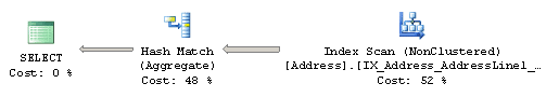
Figure 2 – Graphical execution plan
Physical operators are represented as icons in a graphical plan, such as the Index Scan and the Hash Aggregate physical operators seen in Figure 2. The first icon is called the result operator; it represents the SELECT statement, and is usually the root element in the plan.
Operators implement a basic function or operation of the execution engine; for example, a logical join operation could be implemented by any of three different physical join operators: Nested Loops Join, Merge Join or Hash Join. Obviously, there are many more operators implemented in the execution engine, and all of them are documented in Books Online if you’re curious about them. The Query Optimizer builds an execution plan choosing from these operators, which may read records from the database, like the Index Scan operator shown in the previous plan, or may read records from another operator, like the Hash Aggregate, which is reading records from the Index Scan operator.
After the operator performs some function on the records it has read, the results are output to its parent. This data flow is represented by arrows between the operators, and the thickness of the arrows corresponds to the relative number of rows. You can hover the mouse pointer over an arrow to get more information about that data flow, displayed as a tooltip. For example, if you hover the mouse pointer over the arrow between the Index Scan and the Hash Aggregate operators in Figure 2, you will get the data flow information between these operators as shown in Figure 3.
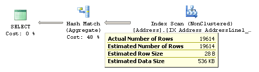
Figure 3 – Data flow between Index Scan and Hash Aggregate operators
By looking at the actual number of rows, you can see that the Index Scan operator is reading 19,614 rows from the database and sending them to the Hash Aggregate operator. The Hash Aggregate operator is, in turn, performing some operation on this data and sending 575 records to its parent, which you can see by placing the mouse pointer over the arrow between the Hash Aggregate and the SELECT icon.
Basically, in this instance, the Index Scan operator is reading all 19,614 rows from an index, and the Hash Aggregate is processing these rows to obtain the list of distinct cities, of which there are 575, which will be displayed in the Results window in Management Studio. Notice also how, in addition to the actual number of rows, you can also see the estimated number of rows; this is the Query Optimizer’s cardinality estimation for this operator. Comparing the actual and the estimated number of rows can help you to detect cardinality estimation errors, which can impact on the quality of your execution plans.
To perform their job, physical operators implement at least the following three methods: Open(), which causes an operator to be initialized, GetRow() to request a row from the operator, and Close() to shut down the operator once it’s performed its role. An operator can requests rows from other operators by calling their GetRow() method. Since GetRow() produces just one row at a time, the actual number of rows displayed in the execution plan is also the number of times the method was called on a specific operator, and an additional call to GetRow() is used by the operator to indicate the end of the result set. In the previous example, the Hash Aggregate operator calls the Open() method once, GetRow() multiple times and Close() once on the Index Scan operator.
In addition to learning more about the data flow, you can also hover the mouse pointer over an operator to get more information about it. For example, Figure 4 shows information about the Index Scan operator; notice that it includes, among other things, data on estimated costing information like the estimated I/O, CPU, operator and subtree costs. You can also see the relative cost of each operator in the plan as a percentage of the overall plan, as shown previously in Figure 2. For example, the cost of the Index Scan is 52% of the cost of the entire plan.
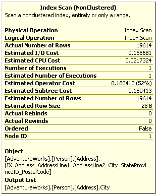
Figure 4 – Tooltip for the Index Scan operator
Additional information from an operator or the entire query can be obtained by using the Properties window. So, for example, choosing the SELECT icon and selecting the Properties Window from the View menu (or pressing F4) will show some properties for the entire query, as shown in Figure 5.
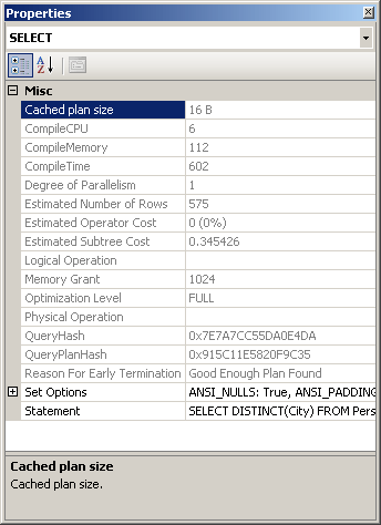
Figure 5 – Properties Window for the Query
Once you have displayed a graphical plan, you can also easily display the same plan in XML format. Simple right-click anywhere on the execution plan window to display a pop-up window, as shown in Figure 6, and select Show Execution Plan XML…; this will open the XML editor and display the XML plan as shown in Figure 7. As you can see, you can easily switch between a graphical and an XML plan.
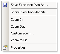
Figure 6 – Pop-up window on the Execution plan window
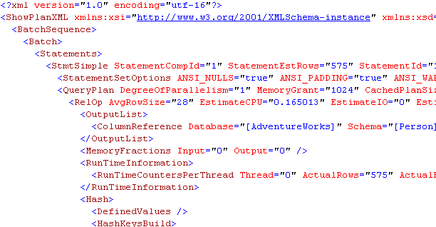
Figure 7 – XML execution plan
If needed, graphical plans can be saved to a file by selecting Save Execution Plan As… from the pop-up window shown in Figure 6. The plan, usually saved with a .sqlplan extension, is actually an XML document containing the XML plan, but can be read by Management Studio into a graphical plan. You can load this file again, by selecting File > Open in Management Studio, in order to immediately display it as a graphical plan, which will behave exactly as before.
Table 1 shows the different statements you can use to obtain an estimated or actual execution plans in text, graphic, or XML format. Note that when you run any of these statements using the ON clause, it will apply to all subsequent statements until the option is manually set to OFF again.
| Estimated Execution Plan | Actual Exection Plan | |
| Text Plan | SET SHOWPLAN_TEXT ON SET SHOWPLAN_ALL ON |
SET STATISTICS PROFILE ON |
| Graphic Plan | Management Studio | Management Studio |
| XML Plan | SET SHOWPLAN_XML ON | SET STATISTICS XML ON |
Table 1 – Statements for displaying query plans
As you can see in Table 1-1, there are two commands to get estimated text plans; SET SHOWPLAN_TEXT and SET SHOWPLAN_ALL. Both statements show the estimated execution plan, but SET SHOWPLAN_ALL also shows some additional information, including the estimated number of rows, estimated CPU cost, estimated I/O cost, and estimated operator cost. However, recent versions of Books Online, including that of SQL Server 2008 R2, indicates that all text versions of execution plans will be deprecated in a future version of SQL Server.
To show an XML plan you can use the following commands:
|
1 2 3 4 5 |
SET SHOWPLAN_XML ON GO SELECT DISTINCT(City) FROM Person.Address GO SET SHOWPLAN_XML OFF |
Listing 2 – Turning on XML execution plans
…Which will display a link starting with the following text:
|
1 |
<ShowPlanXML xmlns="http://schemas.microsoft.com/sqlserver/2004... |
Listing 3 – The result of running Listing 2
Clicking the link will show you a graphical plan, and you can then display the XML plan using the same procedure as explained earlier. Alternatively, you can use the following code to display a text execution plan:
|
1 2 3 4 5 6 |
SET SHOWPLAN_TEXT ON GO SELECT DISTINCT(City) FROM Person.Address GO SET SHOWPLAN_TEXT OFF GO |
Listing 4 – Requesting a text execution plan
This code will actually display two results sets, the first one returning the text of the T-SQL statement. In the second result set you will see the following plan (edited to fit the page), which shows the same Hash Aggregate and Index Scan operators displayed earlier in Figure 2:
|
1 2 3 4 5 |
|--Hash Match(Aggregate, HASH:([Person].[Address].[City]), RESIDUAL ... |--Index Scan(OBJECT:([AdventureWorks].[Person].[Address]. [IX_A ... |
Listing 5 – The result of running Listing 4
Finally, be aware that there are still other ways to display an execution plan, such as using SQL trace (for example by using SQL Server Profiler) or the sys.dm_exec_query_plan dynamic management function (DMF). As mentioned earlier, when a query is optimized, its execution plan may be stored in the plan cache, and the sys.dm_exec_query_plan DMF can display such cached plans, as well as any plan which is currently executing.
The following query in Listing 6 will show the execution plans for all the queries currently running in the system. The sys.dm_exec_requests dynamic management view (DMV), which returns information about each request currently executing, is used to obtain the plan_handle value, which is needed to find the execution plan using the sys.dm_exec_query_plan DMF. A plan_handle is a hash value which represents a specific execution plan, and it is guaranteed to be unique in the system:
|
1 2 3 |
SELECT query_plan FROM sys.dm_exec_requests CROSS APPLY sys.dm_exec_query_plan(plan_handle) WHERE session_id = 135 |
Listing 6 – Displaying the execution plans for currently-running queries
The output will be a result set containing links similar to the one shown in Listing 1-3 and, same as explained before, clicking the link will show you the graphical execution plan. For more information about the sys.dm_exec_requests DMV and the sys.dm_exec_query_plan DMF, you should go to Books Online.
Join Orders
Join ordering is one of the most complex problems in query optimization, and one that has been subject of extensive research since the seventies. It refers to the process of calculating the optimal join order, that is, the order in which the necessary tables are joined, when executing a query. As suggested on the ongoing challenges briefly discussed earlier, join ordering is directly related to the size of the search space as the number of possible plans for a query grows very rapidly depending on the number of tables joined.
A join combines records from two tables based on some common information, and the predicate which defines which columns are used to join the tables is called a join predicate. A join works with only two tables at a time, so a query requesting data from n tables must be executed as a sequence of n – 1 joins, but it should be noted that the first join does not have to been completed before the next join can be started. Because the order of joins is a key factor in controlling the amount of data flowing between each operator in the execution plan, it’s a factor which the Query Optimizer needs to pay close attention to. Specifically, the optimizer needs to make two important decisions regarding joins:
- The selection of a join order
- The choice of a join algorithm
The order in which the tables are joined determines the cost and performance of a query. Although the results of the query are the same regardless of the join order, the access cost of each different join order can vary dramatically.
As a result of the commutative and associative properties of joins, even simple queries offer many different possible join orders, and this number increases exponentially with the number of tables that need to be joined. The task of the Query Optimizer is to find the optimal sequence of joins between the tables used in the query. To clarify this challenge, let’s first clarify the terminology.
The commutative property of a join between tables A and B states that:
A JOIN B is equivalent to B JOIN A.
This defines which table will be accessed first. In a Nested Loops join, for example, the first accessed table is called the outer table and the second one the inner table. In a Hash join, the first accessed table is the build input and the second one the probe input. As we will see, correctly defining which table will be the inner and outer table in a Nested Loops join, or the build input or probe input in a Hash join is important to get right, as it has significant performance and cost implications, and it is a choice made by the Query Optimizer.
The associative property of a join between tables A, B and C states that:
(A JOIN B) JOIN C is equivalent to A JOIN (B JOIN C)
This defines the order in which the tables are joined. For example, (A JOIN B) JOIN C specifies that table A must be joined to table B first, and then the result must be joined to table C. A JOIN (B JOIN C) means that table B must be joined to table C first and then the result must be joined to table A. Each possible permutation may have different cost and performance depending, for example, on the size of their temporary results.
By way of an example, Listing 7 shows a query, taken from Books Online, which joins together three tables in the AdventureWorks database. Click Include Actual Execution Plan and execute the query.
|
1 2 3 4 5 6 7 |
SELECT FirstName, LastName FROM Person.Contact AS C JOIN Sales.IndividualAS I ON C.ContactID = I.ContactID JOIN Sales.CustomerAS Cu ON I.CustomerID = Cu.CustomerID WHERE Cu.CustomerType = 'I' |
Listing 7 – Examining join order
By looking at the resultant execution plan, shown on Figure 8, you can see that the Query Optimizer is not using the same join order as what is specified in the query; it found a more efficient one instead. The join order as expressed in the query is (Person.Contact JOIN Sales.Individual) JOIN Sales.Customer. However, you will see from the plan shown in Figure 8 that the Query Optimizer actually chose the join order (Sales.Customer JOIN Sales.Individual) JOIN Person.Contact.
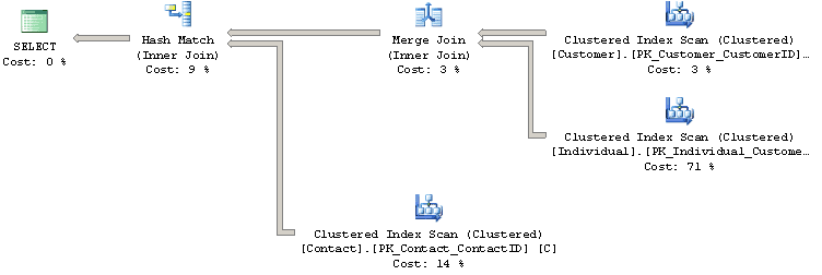
Figure 8 – Execution plan for query joining 3 tables
You should also notice that the Query Optimizer chose a Merge Join operator to implement the join between the first two tables, then a Hash Match join operator to join the result to the Person.Contact table.
Just to experiment, the query shown in Listing 8 shows the same query, but this time using the FORCE ORDER hint to instruct the Query Optimizer to join the tables in the exact order indicated in the query. Paste this query into the same query window in Management Studio as the one from Listing 7, and execute both of them together, capturing their execution plans.
|
1 2 3 4 5 6 7 8 |
SELECT FirstName, LastName FROM Person.ContactAS C JOIN Sales.IndividualAS I ON C.ContactID = I.ContactID JOIN Sales.CustomerAS Cu ON I.CustomerID = Cu.CustomerID WHERE Cu.CustomerType = 'I' OPTION (FORCE ORDER) |
Listing 8 – Forcing a specific join order
The result set returned is, of course, exactly the same in each case, but the execution plan for the FORCE ORDER query (shown in Figure 9), indicates that the Query Optimizer followed the prescribed join order, and this time chose a Hash Match join operator for the first join.
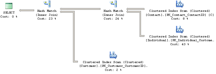
Figure 9 – Execution plan using the FORCE ORDER hint
This might not seem significant, but if you compare the cost of each query, via the Query cost (relative to the batch) information at the top of each plan, you will see that there might be a price to pay for overruling the Query Optimizer, as it has found the hinted query to be more expensive. Specifically, the relative cost of the first query is 38%, compared to 62% for the FORCE ORDER query.
Estimated Subtree Costs
You can get the same result by hovering over the SELECT icon of each plan and examining the Estimated Subtree Cost, which in this case is the entire tree or query. The first query will show a cost of 3.2405 and the second one will show 5.3462. Therefore the relative cost of the second query is 5.3462/(3.2405 + 5.3462)*100 = 62%.
As noted earlier, the number of possible join orders in a query increases exponentially with the number of tables. In fact, with just a handful of tables the number of possible join orders could be numbered in the thousands or even millions, although the exact number of possible join orders depends on the overall shape of the query tree. Obviously, it is impossible for the Query Optimizer to look at all those combinations: it would take far too long. Instead, it uses heuristics, such as considering the shape of the query tree, to help it narrow down the search space.
As mentioned before, queries are represented as trees in the Query Processor, and the shape of the query tree, as dictated by the nature of the join ordering, is so important in query optimization that some of these trees have names, such as left-deep, right-deep and bushy trees.
Figure 10 shows left-deep and bushy trees for a join of 4 tables. For example, the left-deep tree could be:
|
1 |
JOIN( JOIN( JOIN(A, B), C), D) |
And the bushy tree could be:
|
1 |
JOIN(JOIN(A, B), JOIN(C, D)) |
Left-deep trees are also called linear trees or linear processing trees, and you can see how their shapes lead to that description. Bushy trees, on the other hand, can take any arbitrary shape, and so the set of bushy trees actually includes the sets of both left-deep and right-deep trees.
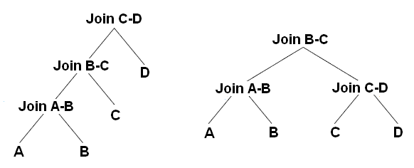
Figure 10 – Left-deep and bushy trees
Table 2 shows how the number of possible join orders increases as we increase the number of tables, for both left-deep and bushy trees, and I’ll explain how it’s calculated in a moment.
| Tables | Left-Deep Trees | Bushy Trees |
| 1 | 1 | 1 |
| 2 | 2 | 2 |
| 3 | 6 | 12 |
| 4 | 24 | 120 |
| 5 | 120 | 1,680 |
| 6 | 720 | 30,240 |
| 7 | 5040 | 665,280 |
| 8 | 40,320 | 17,297,280 |
| 9 | 362,880 | 518,918,400 |
| 10 | 3,628,800 | 17,643,225,600 |
| 11 | 39,916,800 | 670,442,572,800 |
| 12 | 479,001,600 | 28,158,588,057,600 |
Table 2 – Possible join orders for left-deep and bushy trees
The number of left-deep trees is calculated as n!, or n factorial, where n is the number of tables in the relation. A factorial is the product of all positive integers less than or equal to n; so, for example, for a 5-table join, the number of possible join orders is 5! = 5 x 4 x 3 x 2 x 1 = 120.
The number of possible join orders for a bushy tree is more complicated, and can be calculated as:
(2n-2)!/(n-1)!
The important point to remember here is that the number of possible join orders grows very quickly as the number of tables increase, as highlighted by Table 2. For example, in theory, if we had a 6-table join, a query optimizer would potentially need to evaluate 30,240 possible join orders. Of course, we should also bear in mind that this is just the number of permutations for the join order. On top of this, the Query Optimizer also has to evaluate a number of possible physical join operators, data access methods (e.g. Table Scan, Index Scan or Index Seek), as well as optimize other parts of the query, such as aggregations, subqueries and so on.
So how does the Query Optimizer analyze all these possible plan combinations? The answer is: it doesn’t. Performing an exhaustive evaluation of all possible combinations, for a complex query, would take too long to be useful, so the Query Optimizer must find a balance between the optimization time and the quality of the resulting plan. Rather than exhaustively evaluate every single combination, the Query Optimizer tries to narrow the possibilities down to the most likely candidates, using heuristics (some of which we’ve already touched upon) to guide the process.
Summary
This article has covered a lot of ground in a relatively short space, but by now you should have an understanding (or at least an appreciation) of the concepts that are tackled in the book.
We’ve been introduced to the fundamental operations of the SQL Server Query Optimizer, from parsing the initial query to how the Query Optimizer tries to find the best possible execution plan for every query submitted to SQL Server. We’ve also looked at the complexity of the optimization process, including the challenges it faces in exploring the potentially vast search space and accurately estimating cardinality and the cost of candidate execution plans.
As a result of the research that has gone into solving some of those challenges, the Query Optimizer implemented in SQL Server is based on the extensible Cascades Framework architecture, which facilitates the addition of new functionality to the query optimizer, including new operators and transformation rules. Finally, we touched upon the problem of finding an efficient join order in a multi join query, which is still a fundamental challenge in query optimization.
This document contains proprietary information and is protected by copyright law.
Copyright © 2026 Red Gate Software Limited. All rights reserved
Load comments