Uncovering Indexing Problems with Execution Plans

Often, developers will use an Object-Relational Mapping (ORM) tool, such as Entity Framework or nHibernate, to auto-generate SQL code that SQL Server then executes to return the required data. Usually, this approach works well, and the productivity benefits for the developer are obvious. However, it can also result in SQL that returns too much data and has inefficiencies that causes SQL Server to perform far more work than necessary to return the required data. In such cases, the developer needs easy access to SQL Server tools that provide insight into how exactly SQL Server chose to execute their ORM-generated query, and possible causes of poor performance, without dragging them too deeply into SQL Server internals.

One obvious candidate is the SQL Server execution plan. This article serves as a jumpstart into execution plans for the developer who occasionally has to troubleshoot SQL queries that currently don’t perform to specification, and needs deeper insight into the SQL their data access layer generated, and how SQL Server chose to execute it.

It describes what an execution plan is and why it is important, and then looks at some examples of how execution plans can reveal query performance problems relating to missing or poorly-designed indexes, meaning that SQL Server has available inefficient data access paths and performs more IO than necessary to return the required data.

Of course, execution plans can reveal a range of other potential query problems beyond index issues, and subsequent articles will drill deeper into specific problems in SQL, such as ad-hoc queries, data type mismatches, function misuse and so on, which cause excessive reads, plan cache bloat and other problems.

What is an execution plan?

SQL Server executes each SQL query according to a set of instructions called an execution plan, which is devised by a component of the relational engine called the SQL Server Query Optimizer. An execution plan specifies the set of operators required to implement physically each logical step of the submitted query, and the order in which those operations will occur.

Based on information it has about the available data access paths (table, indexes) and statistical information about the data in those tables, the optimizer makes judgements about how much data will be returned from each source, whether indexes are available that will reduce the cost of data retrieval, and so on. Based on these judgements, it selects a plan that it estimates will have the lowest overall execution cost.

Figure 1 shows the graphical execution plan for a simple query against the AdventureWorks2012 database, as viewed in SQL Server Management Studio.

 

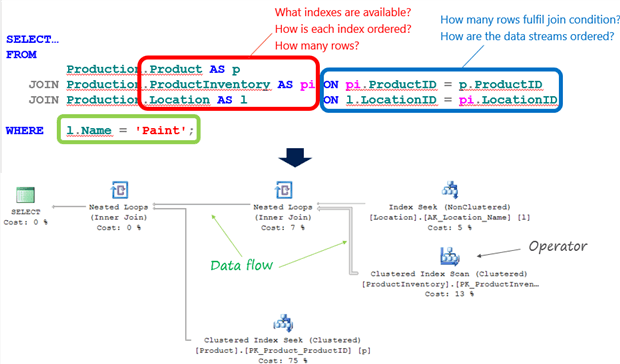
Figure 1

SQL Server has a large set of specialized operators from which to choose, in order to implement each task required in gathering the data and then manipulating it into the correct form to return to the user. Each operator in a plan performs one specific task. The plan in Figure 1 has six operators, connected by arrows, pointing right to left, which represent the flow of data from one operator to the next.

The Basics of Reading Plans

The natural way to read a plan is to follow the data flow, right to left. The two operators on the right-hand side (an Index Seek and Clustered Index Scan), and the one at the bottom (Clustered Index Seek), are data access operators and represent various means of reading the data from the underlying table and indexes.

The optimizer chose first to implement the logical INNER JOIN between the Location and ProductInventory tables, i.e. only returning matching rows, and it chose to implement the join, physically, using a Nested Loops operation, though it can choose other physical join implementations (Hash Match or Merge Join) depending on the number of rows returned and ordering of the data. It seeks an index on the outer table (Location) for 'Paint' and for each row it finds, it uses that row’s LocationID value to perform a search on the inner table (ProductInventory) for matching rows. In this case, it performs a scan of ProductInventory because the available index is ordered on ProductID, not LocationID. The optimizer uses another Nested Loops operation to join this data stream with matching rows in the Product table. Finally, we see a SELECT operator, representing the final result set.

While it’s natural to read a plan right-to-left, the actual execution occurs left-to-right. Each operator supports a method called GetNext(), which is simply a request for a row from the operators immediately to the right. Streaming operators pass on each row, to the left, as it becomes available. All the operators in Figure 1 are streaming. However some operators are partially blocking, meaning they must complete some part of their work before passing on the first row, such as building a hash table in memory (e.g. for a Hash Match join), or collecting all the rows in a grouping set in order to perform an aggregation (e.g. aggregating operators such as a Stream Aggregate), and others, such as a Sort operator, are completely blocking and must collect the entire data set before passing on the first row.

In order to read a plan, we must understand what each operator does and how much data is flowing between each operator. In order to use a plan to uncover possible query problems, we must use the all the information in the plan to understand why the optimizer chose particular operators, and to spot common signs of trouble. This often means that we need to explore the Properties of each operator.

Operator Properties

For each operator, the plan displays a wealth of property values. Some of these properties are operator-specific while others are common to all operators. The plan in Figure 1 (an estimated plan; more on this shortly) shows the properties for the Index Seek operator on the Location table. We can see properties such as the number of rows returned, the number of times the operator was called, various estimated costs associated with executing the operator, the cardinality of the table, and more. Notice that, in this case, the Seek Predicates property shows how our logical WHERE clause was implemented as part for the Index Seek operation.

 

Figure 2

Why Execution Plans are important

Straight away, we can see that an execution plan can reveal very valuable information about how SQL Server chose to execute the query we submitted. In this simple example, we can immediately see the objects accessed by the query and the order in which they were accessed, which indexes were used (or not), and how joins were implemented. In more complex queries, the plan would also reveal when sorting occurred, how calculations and aggregation were performed, and more. If we know how to read a plan and can mine the information they divulge, we use the plans to look for common signs of potential trouble, which lead to poor query performance.

More fundamentally, the mere existence of a component called the Query Optimizer tells us that SQL Server, not the database developer, decides how a query should be executed. We submit an SQL query to describe the required set of data. We do not tell SQL Server how to execute it. The optimizer is completely free to choose the set of operators for the plan, and set their order, within the overriding requirement that the resulting plan must guarantee to return exactly the same data set as would be returned according to the logical processing order of the query. Except for very simple queries, the physical processing order, as expressed in the plan, will likely not match the logical processing order. We saw a very simple example of this with the previous example. Logically, the processing order of the WHERE clause comes after the FROM clause, but in practice it is more efficient to “push down” the predicate and retrieve only the rows that match the predicate condition, rather than retrieve all the rows and then filter out those that are not required.

In the vast majority of cases, decisions on processing order should be left entirely in the hands of the optimizer. Developers need to be wary of bringing to SQL Server their standard, imperative approach to programming, with line-by-line control over what happens and when. It can lead to sub-optimal plans and poor performance. We won’t discuss this further here, but Peter Larsson, who writes SQL most can only dream of, explores these ideas in more detail in this article.

How the optimizer generates plans

When a query reaches the relational engine, it is parsed by the Parser, bound by the Algebrizer and then optimized by the Query Optimizer. Collectively, these processes are referred to as query compilation i.e. the process of compiling a query into an execution plan.

The optimizer generates a number of candidate execution plans for each query submitted, and chooses the plan that it estimates will have the lowest overall execution cost in terms of CPU and IO. Of course, the optimizer cannot actually execute any queries, so its cost estimates and subsequent plan choices are based on its knowledge of the underlying data structures (i.e. the tables and available indexes), and on statistics, aggregated information based on a sample of the data, describing the volume and distribution of data in those data structures.

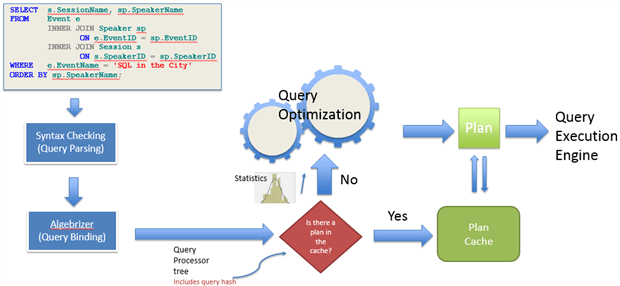
Figure 3

The optimizer’s cost estimates depend largely on its cardinality estimations, of how many rows are in a table, and how many of those rows satisfy the various search and join conditions.

It uses all this information to answer questions such as:

• How many rows in the table?
• How many rows match the search condition?
• What indexes are available?
• How is each index ordered?
• What is the index density?
• How many rows match the join conditions?
• How are each of the required data streams ordered?

Based on its knowledge and estimates, the optimizer chooses the most efficient data access path and the most appropriate operators to implement each phase of the query.

The optimizer’s selected plan passes to the query execution engine, and is also stored in an area of memory called the plan cache. The next time we submit the same query, SQL Server may be able to reuse an existing plan in cache, rather than generate a new one, and therefore bypassing the optimization phase. We’ll tackle the topic of plan reuse in a later article.

Viewing Execution Plans

SQL Server stores execution plans in the plan cache, in a binary format. SQL Server can output these plans in XML format (recommended) or in text format (deprecated). When viewing execution plans in SQL Server Management Studio (SSMS), and in some third party tools, we can see a visual representation of the XML, called a graphical plan (see Figure 1). Graphical plans are most common format in which to read execution plans, and are the only format presented in his article.

View graphical plans in SSMS

In SSMS, we can view an execution plan with or without runtime information. The version of the plan without runtime information is called the estimated execution plan, and the version with runtime information is called the actual execution plan.

 

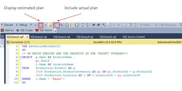
Figure 4

When we request to display an estimated plan for a query, the optimizer performs the parsing and binding phases, and then the optimization phase, assuming no there is no plan it can reuse in the cache, as described in Figure 3. However, it does not execute the query (no result set will be returned). Therefore, all property values displayed with the plan, and for each operator, such the number of rows returned, the number of times the operator was called, and the various costs associated with executing the operator, are all estimates. Estimated plans are useful during development for testing large, complex queries that could take a long time to run.

If we request what SSMS refers to as the “actual plan”, it means we wish to execute the query. Upon completing execution, SQL Server has available certain runtime information, namely the actual number of rows and actual number of executions, which it can display with the plan. All costs associated with the operators are still estimates.

Use the SET options to return XML plans for a session

We can use SET statements to return the execution plan in XML format, again either with or without runtime statistics:

• SET SHOWPLAN_XML ON | OFF – returns “estimated” plans (no runtime information); no T-SQL statements are executed
• SET STATISTICS XML ON | OFF – executes the queries and returns the plan with runtime information (the “actual” plan)

Plans will be returned for all statements executed in the session, until the option is turned off. A common problem for developers who don’t have access to SSMS, or don’t want to use it, is that they don’t have an easy way to read and interpret the XML plan.

One solution is to use a free web-based tool called SQL Tune Up, available through SQLServerCentral.com. Simply drop the execution plan file (.sqlplan) onto the page, and it will display it as a graphical plan.

This functionality is built into the ANTS Performance Profiler tool, which we’ll cover shortly.

Retrieve the cached plan

We can use a variety of tools, such as Extended Events or SQL Trace, to retrieve from the plan cache the plans for previously-executed queries. I won’t cover these tools in this article. We can also retrieve the cached plan by querying the sys.dm_exec_cached_plans dynamic management object (a little more on this shortly).

Use a Code Profiling tool

A commercial code profiling tool such as Red Gate’s ANTS Performance Profiler (APP) exposes expensive methods in your .NET application code. The latest version of the tool also exposes expensive SQL calls, and allows the developer to drill into these expensive data operations and examine cached execution plans for these queries. It means that developers who use the tool now have a way to troubleshoot side-by-side bottlenecks in both the .NET code and in the SQL code.

The Index Operators in Execution Plans

I won’t cover heaps in this article; in other words, I’ll assume that all tables have a clustered index, which is a generally-accepted best practice, except for some small tables with a very high read:write ratio. In addition to a clustered index, most tables will have a number of non-clustered indexes, designed to aid the performance of critical, frequent and expensive queries in the workload.

There are essentially three ways that SQL Server can access data in an index:

• Seek – navigate directly to the page(s) containing the qualifying rows or the start/end of a range of rows.
  • Execution Plan Operators:

Clustered Index Seek

Index Seek (NonClustered)

• Scan – navigate down to first or last leaf level page of the index and then scan forward or backward through the leaf pages. A scan usually reads the entire index, but may read only a portion of the index in some cases.
  • Execution Plan Operators:

Clustered Index Scan

Index Scan (NonClustered)

• Lookup – occurs in addition to an Index Seek or Index Scan, when the index is non-covering. SQL Server performs a key lookup to the clustered index to retrieve values for columns not available in the non-clustered index.
  • Execution Plan Operator:

Key Lookup (Clustered)

Clustered Index Seeks and Scans

Indexes consist of 8K pages connected in a B-tree structure. Figure 5 represents a simplified view of the B-tree structure for a simplified version of the clustered index on the SalesOrderDetail table of the AdventureWorks2012 database. In this version the clustering key is SalesOrderID (in reality the clustered index uses a composite key on SalesOrderID and SalesOrderDetailID). There are 120K rows in the table.

 

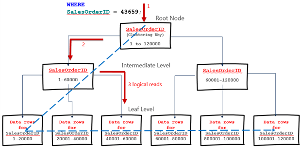
Figure 5

A clustered index is not a “copy” of the table. It is the table, with a b-tree structure built on top of it, so that the data is organized by the clustering key. This is why we can only create one clustered index per table.

The leaf level pages of a clustered index store the data rows, ordered according to the clustering key. In Figure 5, a query requests the row for a specific SalesOrderID value, and SQL Server navigates the b-tree structure directly to the page containing that row, as represented by the orange arrows. This results in a clustered index seek operator in the execution plan. Each page it needs to read in order to retrieve the data represents a logical read, so in this case it can return the data in 3 logical reads.

If, instead, our query searches for a row based on a column value other than SalesOrderID, such as CarrierTrackingNumber then assuming there isn’t a non-clustered index on CarrierTrackingNumber, nor a covering non-clustered index that it could scan, SQL Server will scan the clustered index.

It will navigate down to the first leaf level page of the clustered index and then scan all subsequent leaf pages looking for matching rows. This is a clustered index scan, as represented by the blue, dashed arrow in Figure 5. The number of logical reads to return the data will likely be the number of leaf level pages in the index (plus the root and any intermediate pages). In Figure 5, each leaf level page stores 20K rows, which is unrealistic. Each leaf page in the figure might represent 100 leaf pages in a real index (i.e. 200 rows per page and 600 logical reads in a scan of an index of this size, although these are just ‘ballpark’ figures).

Sometimes, scans are highly efficient operations, especially for queries that return a substantial proportion of the table data. However, a general goal for critical and frequently-executed queries is to have non-clustered indexes in place that will allow SQL Server to seek the required data in as few logical reads as possible.

Index Seek and Scans, plus Key Lookups

A non-clustered index has the same b-tree structure, but the difference is that the leaf level pages do not contain the data rows, just the data for the index key columns, plus the clustered index key columns, plus any columns that we add to the index using the INCLUDE clause.

Figure 6 shows a simplified depiction of a non-clustered index on the ProductID column of the SalesOrderDetail table. The index has no INCLUDE columns. The leaf pages contain only the values for the index key column (ProductID) and the clustered index key columns (SalesOrderID).

 

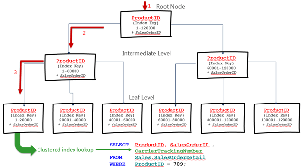
Figure 6

If SQL Server uses this index for a query that searches on a column other than ProductID, it will result in an Index Scan (as described previously for clustered index scan). If a query searches on ProductID, and only requires this and the SalesOrderID values, then SQL Server will perform an Index Seek. If the query searches on ProductID, but also requires additional columns, such as CarrierTrackingNumber, then we will see in the plan an Index Seek plus a Key Lookup operator, where SQL Server will look up in the leaf level of the clustered index the matching values for CarrierTrackingNumber.

Other Useful Tools for Index Investigation

I will mention briefly here, but not cover in any detail, a few tools that I find useful when investigating further any potential indexing problems that I uncover through the execution plans. The first, which I use in this article, is Michelle Ufford’s Estimating rows per page script, as reproduced in Listing 1.

Listing 1

For critical queries, I find the data useful in providing a “target” number of logical reads, depending on the rows-per-page and the number of rows the query needs to return. I also recommend many of the other index-related scripts, and others, in Michelle’s archive (now open-sourced).

Kimberley Tripps’s version of sp_helpindex, an improved version of the tool of the same name on MSDN, is also very useful for investigating the various indexes on your tables and their structure

The index-related Dynamic Management Views provide a wealth of information regarding existing indexes and their usage statistics, as well as potentially missing indexes. There are numerous excellent community-supplied scripts available that mine the information in these objects, some of which I reference in Further Reading, at the end of the article.

One approach I find particularly useful during testing is to use these objects to search the plan cache for existing plans for queries that caused expensive scans. I can then examine the plans to see which columns are involved in the searches and joins for those queries, and look for indexing opportunities.

Investigating Indexing Issues with Execution Plans

This section will provide some examples that demonstrate how to spot signs of potential SQL Server indexing problems in the execution plan. The examples are simple and the target tables quite small, meaning that indexing becomes less critical. Nevertheless, they do illustrate some of the thought processes behind sensible indexing, which will apply for larger tables.

It will cover issues such as:

• Choice of clustered index – ideally narrow, static, ever-increasing but establishing the “natural order” of the data.
• Missing non-clustered indexes – to support Foreign Key columns, common searches, aggregations and so on.
• Why SQL Server may chose not to use a non-clustered index – if the index is non-covering and not selective enough for the key lookups to be efficient.

We’ll focus on the details of the plans, and provide references for further reading on the broader topic of general indexing strategies for SQL Server databases.

ANTS Performance Profiler and the LibraryManager Application

The examples in this article use ANTS performance Profiler (APP) to view the execution plans, along with an internal LibraryManager application, which by design has a few application performance problems, introduced to help illustrate functionality in ANTS Performance Profiler. Library Manager is an admin console that could be used at a library. It is built with WinForms and Entity Framework and uses a SQL Server database called LibraryManager.

As part of the code download you will find the .sln file for a simple web form that will run the LibraryManager queries that we investigate in the article, against the LibraryManager database. You will just need to update the App.config file with the connection string to your database server, build the solution in Visual Studio, and then start up APP and attach to the executable (in the debug folder). You’ll also find a database backup file (.bak), which you can restore to create the LibraryManager database.

Alternatively, in the code download file you’ll find SQL code files that will allow you to run the queries in SSMS, if you prefer, in which case you will simply need to create a copy of the LibraryManager database.

Getting Started

If you wish to use APP, fire it up, define a New profiling session and attach to the LibraryManager application by entering the path to the executable. Make sure you choose the Line-level and method-level timings.

Upon startup the LibraryManager application automatically fires off a selection of queries to the database, so we see some immediate action in APP (you won’t see exactly the same queries executed each time you start or restart a profiling session).

The top third of the screen shows the activity timeline including, at the top, an adjustable sliding region control, which we can use to focus on a specific area of interest on the timeline. APP continues collecting diagnostic data, in the background, while we focus in on a specific region. We can use bookmarks to save interesting regions, so we can always jump back to that regions as APP continues to collect profiling data.

 

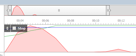
Figure 7

The lower portion of screen shows, by default, the call tree view of application activity, in other words the various method calls made in the selected time period, and their timings.

 

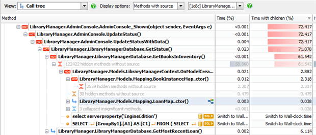
Figure 8

We can see immediately several “hot” (expensive) .NET methods, which we’re going to ignore in this article, since we’re focusing in on database calls. The important point is that we’re seeing expensive SQL calls right alongside the expensive .NET methods.

By default the timings show CPU time as a percentage of total cost of all method calls in that time window. For SQL calls, we need to switch the timing options to Wall-clock time and Milliseconds. Also, the timing switch occurs automatically if we select the Database calls view, as shown in Figure 9.

 

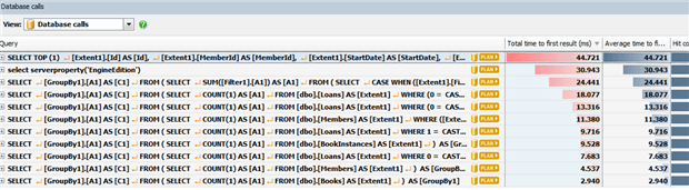
Figure 9

Let’s investigate the most expensive queries, using execution plans, since some of them could benefit from more efficient indexing.

Clustered Index operations

The design the clustering index is mainly from the perspective of organizing the table. The key characteristics of a clustering key, as discussed in many articles (see Further Reading), are for it to be narrow, static and ever-increasing. For this reason, many clustered indexes tend to use an IDENTITY column as the clustering key. However, date-based columns are often useful clustering keys in OLTP databases, particularly when the data is commonly-queries by date ranges.

Let’s consider our first example. The most expensive query currently identified for our LibararyManager application returns various details relating to the most recently loaned book.

Listing 2

The application uses Entity Framework to generate these queries. The code download file provides “sanitized” version of these queries, minus the Entity Framework-generated clutter.

One point to notice is that this is effectively a “SELECT *” query, returning every column in the table. This makes the task of creating effective indexes much harder. If possible, limit the columns returned to only those that are really required.

Click on the Plan button to reveal how the SQL Server Query optimizer chose to execute this query. You may have to enter Windows or SQL credentials to connect to the target instance. Above the plan you’ll see a note (not shown in Figure 9) that the plan is a cached execution plan, meaning the plan generated by the query optimizer and stored in the plan cache. As discussed earlier, all row-, execution- and cost-related properties for this plan will be estimated values, based on statistics. If we were to copy the query text from Listing 2 into SSMS and execute it, selecting Include Actual Execution Plan, we will see the same plan, but this time with actual row number and execution counts alongside the estimated ones.

 

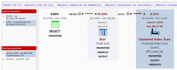
Figure 9

The query accesses only one table, the Loans table, and we can see that the optimizer opted to access the data via a Clustered Index Scan. In other words, it scanned all the pages in the leaf level of the clustered index, PK_Loans_Id. The Loans table has 24693 rows, as indicated by Table Cardinality in the PROPERTIES link below the Clustered Index Scan operator. This scan operation passes on the 22352 rows that match the predicate condition.

The TopN Sort operator, which combines both Sort and Top operations, sorts the data in order of descending StartDate and then selects only the top row, which it passes to the SELECT operator.

APP provides some “sugar coating” to the plans that we would normally see in SSMS. It makes the estimated IO and CPU costs and number of rows immediately visible, so that we don’t have to dig through the each operator’s Properties window to see them. For each operator certain key properties appear in separate links, again to make the information more easily accessible. For example, if we click the PREDICATE link for the scan, we’ll see that the search predicate in our WHERE clause was “pushed down” into this operator.

 

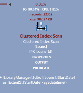
Figure 10

APP also highlights in red boxes, to the left of the plan, expensive and “data heavy” operations, the Sort and Clustered Index Scan respectively, in this case. The Sort is a blocking operation. It must collect all 22352 rows, sort them, before passing on the first row. In this case, the first row is only one the query requires.

The second problem, potentially, is the clustered index scan. Currently the clustered index key is the Id column, an IDENTITY column. While this column fulfils the preferred criteria for a clustering key, it offers no support for searches based on date, which are common, and there are no searches on Id in the workload. The current query sorts on StartDate, and uses StartDate in a search predicate.

Let’s collect execution statistics for Listing 2.

We see 146 logical reads to return the data, with 40 ms elapsed time.

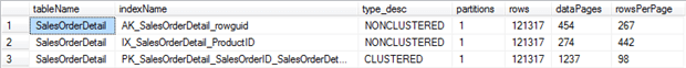
Figure10 shows the output from the data-rows-per-page script (Listing 1) for the Loans table in the LibraryManager database.

 

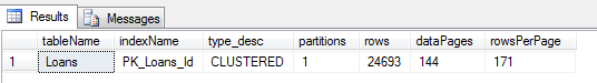
Figure 10

The PK_Loans_Id clustered index contains 144 data pages (leaf level pages) with an average of 171 rows per page. Our index is 2-levels deep (you can check this using the index_depth column in the sys.dm_db_index_physical_stats DMV). SQL Server scans every leaf-level page of PK_Loans_Id, plus the root page (plus the Index Allocation Map page) for a total of 146 logical reads. Ultimately, we only return only a single row.

Clearly, it would be beneficial to have an index ordered by StartDate. One solution might be to create a non-clustered index on StartDate, but then that index would need to include all of the required columns, if we wished to avoid Key Lookups (covered later).

If searches based on StartDate are very common in our library application, then another option is to reconsider the choice of clustered index key for this table, and instead use StartDate as the clustered index key. Alternatively, you might decide to create a composite key on (StartDate, ID). In the former case, SQL Server will add a “uniqueifier” to duplicate key values. The uniqueifier is an INT, so it’s more overhead than adding the IDENTITY column to the clustered index.

Listing 3

If we re-execute Listing 2, capturing new execution statistics, we see a big difference; only 2 logical reads to return the row we require instead of 146.

If we re-run the APP profiling session on LibraryManager, we will see that the query in Listing 2 has now slipped well down the list of expensive queries. The execution plan reveals a Clustered Index Seek, in place of the scan and that we no longer need the expensive Sort operation, since the data can be retrieved from the clustered index in the correct order.

 

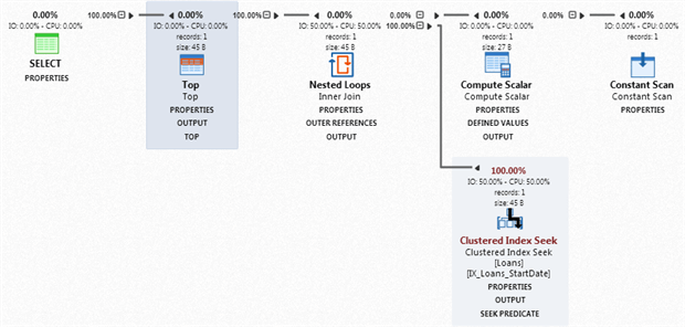
Figure 12

The Compute Scalar and Constant Scan operators represent calculation or conversions (related to use of SysDateTime in this case). If you open the Properties for the Clustered Index Seek, you’ll see that the Scan Direction is BACKWARD, since the index is organized in ascending order with respect to StartDate, so SQL Server searches it backwards, to get the most recent date. It’s not really a concern for this query, but note that backwards scans cannot be parallelized. We could have considered created the clustered key as StartDate DESC, but this can cause index fragmentation.

Of course, this index will also support broader queries in the workload based on StartDate, such as searches for all loans in the past 12 months (WHERE StartDate >= DATEADD(MONTH, -12, CURRENT_TIMESTAMP)).

Adding Non-Clustered Indexes

Having chosen carefully the clustered index for each table, the next task is to choose the set of non-clustered indexes that will best serve the critical queries in your workload. Our goal is to design a minimum set of non-clustered indexes that will support our most frequent (i.e. executed many time per day) and most business-critical queries. Find out how those queries filter, and then create a set of indexes such these queries filter (or join, or aggregate) on a left-based subset of the index key.

We need to avoid the tendency to index every column “just in case”, which could destroy the performance of data modifications on that table, since every time we modify a column, SQL Server must all modify all indexes in which that column participates. If a query has multiple conditions in the WHERE clause, it is far better to create one index that contains all of these columns (the order might be important) than to create separate indexes on each column.

Let’s look at the next most expensive query in our list.

Listing 4

Entity Framework’s “ultra-conservative” mode of SQL generation makes this query look a little more complex than it really is. It is equivalent to Listing 5 and simply calculates the sum of unpaid fines.

Listing 5

Here is the execution plan for Listing 4, from APP.

 

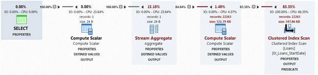
Figure 13

To return this data SQL Server scans every leaf-level page in the clustered index (146 logical reads in total, as before) and returns the 22263 rows where FinePaid is 0. The PREDICATE for the scan shows an explicit data type conversion of FinePaid to an int (the underlying data type of the column is tinyint). Listing 5 avoids this conversion.

The DEFINED VALUES for the first Compute Scalar operator indicates that for each of the 22263 rows returned, it performs an implicit conversion of the FineIncurred column from money to decimal(22,4) and assigns the resulting value to a variable called ExprXXXX. Running the simplified query in Listing 5 eliminates both this and the previous explicit conversion. The Stream Aggregate operator performs our SUM aggregation and will ignore any NULL values in FineIncurred.

If we refine the WHERE clause in our query in Listing 4 or 5 to discount rows with NULL values for FineIncurred, by adding AND FineIncurred IS NOT NULL, then the plan remains the same except the scan returns only 51 rows, which reduces the cost of the aggregation slightly (to 14%).

For the query in Listing 4 (or 5), the missing index advisor in SSMS pops up and suggests an index that we might like to create to increase the performance of this query. APP exposes this as a “warning” that SQL Server has detected an index that could reduce the cost of the query by 77%.

 

Figure 14

Listing 6 shows the script for the suggested missing index.

Listing 6

I have mixed feelings about seeing this raised in APP as a “warning”, because it is well-documented in many online articles (see Further Reading section) that the suggestions of the missing index advisor, as well as the data mined directly from the missing index Dynamic Management Views, should be treated as a guide only. Your indexing strategy should be considered in relation to the workload as a whole, and certainly it’s a bad idea to create every index suggested by the advisor, as you will end up with a lot of duplicate or very similar indexes.

Nevertheless, in this case, let’s accept the advice and create the index. I won’t reshow the plan, but you will find that the clustered index scan is replaced by an Index Seek on the new index. Collecting execution statistics will reveal that the number of logical reads is down from 146 to 77. Rerunning Listing 1 reveals that the new index has 83 data pages (297 rows per page). The seek operation traverses the vast majority of these pages simply because most of the entries in FinePaid are 0.

Generally, I’d question the overall benefit of such an index, unless this happened to be a query that ran very frequently. The problem is that the majority of the values in the FineIncurred column are NULL (only 2481 are non-NULL), and therefore the corresponding FinePaid values for all of these entries is 0. It could be beneficial in cases such as this one to use a filtered index (first, drop the existing index on FinePaid).

Listing 7

The filter in a filtered index must match or be a superset of the filter in a query. This index only has 9 leaf level pages and SQL Server only needs to read one of them to retrieve our data (we see a total of 3 logical reads).

As with any index, before creating a filtered index you would want to check the workload and ensure that it’s useful in general and not for one specific query.

Lookups and non-covering indexes

The Query Optimizer makes it choices about which indexes will be useful based in large part on the density of the index and selectivity of the predicate.

A unique index has the lowest possible density and equality predicates against a unique index have the highest possible selectivity, since if we search it for a particular value we are guaranteed to return one row. Conversely, columns such as “Gender” or the FinePaid column from the previous example have relatively high density; searches on the index are likely to return many rows.

If an index is non-covering, i.e. doesn’t hold all the column values that a query requires, then whether or not the optimizer opts to use it will depend on estimated selectivity of the predicate.

Here’s a third query from our LibraryManager list, followed by its simplified equivalent.

Listing 8

I won’t show the plan again, since it’s simply a clustered index scan of IX_Loans_StartDate, which again causes 146 logical reads. Let’s assume we decide to cover the query with an index.

Listing 9

Now, the plan for our query will show an index seek. However, will other queries in our workload be able to make use of this index? For example, consider the query in Listing 7 to see all loans that are due to be returned in the next 2 weeks.

Listing 10

The Optimizer estimates that 34 rows will be returned out of 24693 (about 0.014%). This is selective enough that the optimizer will use the index, even this it is not covering for this query, and then perform a key lookup to the clustered index to retrieve values for the remaining columns. As you can see from the actual execution plan in Figure 15, captured this time in SSMS, it actually only returns 6 rows.

 

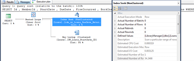
Figure 15

However, there is a low “tipping point” at which the optimizer will switch to ignoring our index and instead scanning the clustered index. For example, extending the search to books due to be returned in the next month results in a clustered index scan, along with a suggestion to create an index to cover the query (which would make our previous index redundant).

 

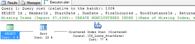
Figure 16

Again, generally, it would be unwise, for reasons previously discussed, to attempt to “cover” every query. However, of course, we should create indexes to cover our most frequent and important queries.

Summary

When you start to write SQL Queries, you are likely to assume that you are specifying not only the result that you want, but the way that the Relational Databases should fetch the rows. This isn’t the case. In SQL Server, the query optimizer determines the best way of executing the query, based on the evidence it has. The same query can be executed in many different way as the data size increases, new indexes become available, or as the data distribution changes. You can influence the optimizer by applying hints, but you’d be hard put to do better than the optimizer. However, you can easily make life difficult for the optimizer in a number of ways, such as failing to provide the right indexes to support the query, or by preventing the optimizer from estimating the size of intermediate results properly. To ensure that your queries are ‘kind’ to the optimizer, and are likely to perform well no matter how much data is in the tables, it is essential to be able to understand execution plans.

Further Reading

Choosing Clustered Index Key

• Effective Clustered indexes – a good explanation of the key design principles for the clustered indexhttps://www.simple-talk.com/sql/learn-sql-server/effective-clustered-indexes/
• GUIDs as PRIMARY KEYs and/or the clustering key – why GUIDs make very bad clustered index keyshttp://www.sqlskills.com/blogs/kimberly/guids-as-primary-keys-andor-the-clustering-key/
• Clustered Index Design Guidelines – advice from Books Online:https://technet.microsoft.com/en-us/library/ms190639(v=sql.105).aspx

General Indexing Considerations

As general resources, I recommend the Index section of the blogs of Gail Shaw (http://sqlinthewild.co.za/index.php/category/sql-server/indexes/) and Kimberley Tripp (http://www.sqlskills.com/blogs/kimberly/category/indexes/).

See also:

• Nonclustered Index Design Guidelines – advice from Books Onlinehttps://technet.microsoft.com/en-us/library/ms179325(v=sql.105).aspx
• SQL University: Advanced Indexing – Indexing Strategies http://sqlinthewild.co.za/index.php/2011/11/11/sql-university-advanced-indexing-indexing-strategies/
• One wide index or multiple narrow indexes?http://sqlinthewild.co.za/index.php/2010/09/14/one-wide-index-or-multiple-narrow-indexes/
• Are your indexing strategies working? (aka Indexing DMVs)http://www.sqlskills.com/blogs/kimberly/the-accidental-dba-day-20-of-30-are-your-indexing-strategies-working-aka-indexing-dmvs/
• Don’t just blindly create those “missing” indexes!http://sqlperformance.com/2013/06/t-sql-queries/missing-index
• Query Tuning Fundamentals: Density, Predicates, Selectivity, and Cardinalityhttp://blogs.msdn.com/b/bartd/archive/2011/01/25/query_5f00_tuning_5f00_key_5f00_terms.aspx

Filtered Index Design Guidelines

• Filtered Index Design Guidelineshttps://technet.microsoft.com/en-us/library/cc280372(v=sql.105).aspx
• SQL University: Advanced Indexing – Filtered Indexeshttp://sqlinthewild.co.za/index.php/2011/11/09/sql-university-advanced-indexing-filtered-indexes-2/