
R is an extremely versatile statistical analysis platform. It is designed to perform complex calculations using only a few interactive commands or a short script. Many R users initially use the language to create a statistical summary or chart using a tiny subset of the available functionality. The R-Basics and Visualizing Data with R articles introduce these topics, but don’t go into much detail about how to manipulate datasets within R.
A subsequent article describes the use of SQL and R for interacting with databases and manipulating data frames. The R community has created a number of SQL-related packages available from CRAN (the Comprehensive R Archive Network). Many of these allow R to query and process data in relational databases, but others (like sqldf) can be used with data that does not explicitly originate in, or target, a relational database. The availability of SQL within R is incredibly valuable for many data problems, particularly if you “think” in SQL. A dataset can be conveniently sorted, filtered, manipulated, re-ordered and analyzed. These basic operations are intrinsic to SQL and applicable to any dataset that conforms to the “shape” of a standard database results set.
SQL is a well-understood standard language that is familiar to many developers and analysts. It is used in most modern relational databases and has influenced similar query languages on non-relational platforms. R syntax can be confusing when initially encountered, so if you are comfortable using SQL, you can use it to jump-start your development on R.
Although SQL is a popular way to process data frames, there are situations where a different approach is warranted. Certain data transformations are notoriously difficult to express using SQL. Such transformations require complex, obscure syntax or multiple statements executed in sequence. The core R programming language and a number of publicly available packages can be leveraged to easily accomplish such tasks.
Complex SQL Not Required
Operations that are conceptually simple can be difficult to perform using SQL. Consider the common requirements to pivot or transpose a dataset. Each of these actions are conceptually straightforward but are complex to implement using SQL. The examples that follow are somewhat verbose, but the details are not significant. The main point is to illustrate is that, by using specialized functions outside of SQL, R makes trivial some of those operations that would otherwise require complex SQL statements. The contrast in the amount of code required is striking. The simpler approach allows you to focus attention on the scientific or business problem at hand, rather than expending energy reading documentation or laboriously testing complex statements.
Example 1: The Pivot
Pivoting a table (also known as cross tabulation) involves transforming certain data elements into columns. This task will introduce the reshape2 package. If you are following along and have not installed the package, you will have to do so using the RStudio GUI or at the command prompt by running.
|
1 |
install.packages('reshape2') |
Once installed, the library needs to be included in the current R session.
|
1 |
library(reshape2) |
Note that an earlier less optimized package named “reshape” provides similar functionality and a corresponding API. It’s will not be used in the examples that follow.
Many relational databases have PIVOT and UNPIVOT functions to create a crosstab report. Examples using SQLServer are presented in other posts on Simple-Talk. This syntax is consistent with other RDBMS implementations. Consider a results set returned by a query on Oracle’s HR demonstration schema.
|
1 2 3 4 5 |
select job_id, department_name, sum(salary) salary from DEPARTMENTS d join EMPLOYEES e on e.DEPARTMENT_ID = d.DEPARTMENT_ID where job_id in ('ST_MAN','AD_ASST','PU_MAN','SH_CLERK') group by job_id, department_name; |
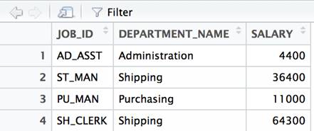
The results represent the total salary for a given job title within a department.
|
1 2 3 4 5 |
JOB_ID DEPARTMENT_NAME SALARY AD_ASST Administration 4400 ST_MAN Shipping 36400 PU_MAN Purchasing 11000 SH_CLERK Shipping 64300 |
You can create a dataframe in R to hold this data and view it as follows:
|
1 2 3 4 5 6 7 8 |
df<- data.frame( JOB_ID=c('AD_ASST','ST_MAN','PU_MAN', 'SH_CLERK'), DEPARTMENT_NAME = c('Administration','Shipping','Purchasing','Shipping'), SALARY=c(4400, 36400, 11000, 64300) ) View(df) |
The View() command is used to provide the spreadsheet-like view of the data. It will be omitted in subsequent examples. Any example that returns data can simply be wrapped in a View() method call to be viewed in this manner.
A pivot operation applied to the operation results in each department name being used as a column. Essentially, the original query is wrapped in and a pivot clause is appended. The pivot clause lists the data value and column names to use.
|
1 2 3 4 5 6 7 8 9 10 11 12 |
select * from (select job_id, department_name, sum(salary) salary from DEPARTMENTS d join EMPLOYEES e on e.DEPARTMENT_ID = d.DEPARTMENT_ID where job_id in ('ST_MAN','AD_ASST','PU_MAN','SH_CLERK') group by job_id, department_name) pivot ( sum(salary) for (department_name) in ( 'Administration', 'Purchasing', 'Shipping') ) order by 1; |
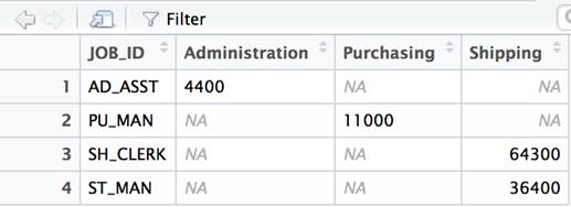
The results contain the same data presented in a pivot format.
|
1 2 3 4 5 |
JOB_ID Administration Purchasing Shipping AD_ASST 4400 PU_MAN 11000 SH_CLERK 64300 ST_MAN 36400 |
Earlier SQL developers devised clever but notoriously complicated solutions before the PIVOT function was implemented. Some relied upon non-standard database specific functionality while others required several queries to be executed to create intermediate results before creating the final crosstab report. The PIVOT function is an improvement, but remains a fairly verbose option when compared with the ability to “cast” a database using a function from the reshape2 package.
|
1 |
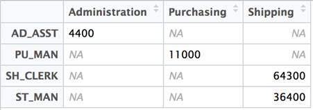
df2<- dcast(df, JOB_ID ~ DEPARTMENT_NAME) |
Example 2: The Transpose
Transposing a dataset involves rotating a result set so that the rows from the original result set are columns in the final result set. This relatively simple idea is surprisingly difficult to express in SQL (though it is certainly possible). No special packages are required. The R base language contains a built in transpose function. We could just proceed to transpose, but the dataset as represented has an inconsistency. The column names are not part of the dataset, but the row names are. SQL has a concept of column names but not row names. Our results will be a bit neater if we assign row names based on JOB_IDs and remove the JOB_ID column from the data. These two statements enact these changes.
|
1 2 3 |
rownames(df2) <- df2$JOB_ID df2<-df2[-1] |
We will pause here for a moment to consider a few aspects of R that are a bit surprising. Most programming languages do not support a function call on a variable that is the recipient of an assignment, yet R allows you to return the row names of the data frame and use the returned value as the recipient of an assignment. In addition, most languages require that each item in a collection be assigned individually. This often requires a looping construct to iterate through each available assignment target and value. R, being vector based, allows the set of row names associated with the data frame to be assigned all at once.
The second line shows one of several methods available to remove a column. In this case, the minus sign indicates a column should be deleted. R, being one-based rather than zero based like many other programming languages, interprets this to mean “return a data frame like the current data frame without the first column.” This value is then assigned back to the variable that held the original reference to the data frame.
The net effect is that the first column disappears from the dataset and row names are now associated with the data frame.
The idea of transposing a matrix is a well-understood concept in linear algebra and is commonly used in statistical analysis. Since it has a long history of providing statistical functions, R included matrix manipulation from its earliest days. All that is required to flip the data frame is to call the t function.
|
1 |
t(df2) |
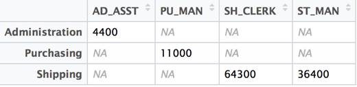
That’s all there is to it! There are some limitations. But in this case, with consistent numeric data and column and row names outside of the dataset proper, the conversion works as expected. Lets look at a different example where the limitations become evident.
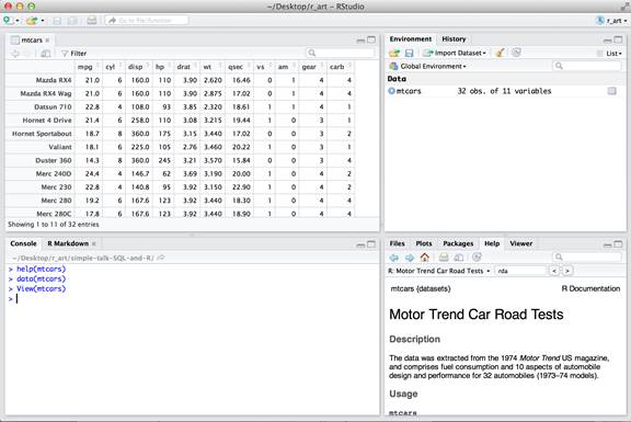
Recall the “mtcars” dataset introduced in a previous post that is derived from 1974 Motor Trend US magazine data (hence the “mt” in the dataset name). The dataset describes fuel consumption and various aspects of automobile design and performance for 32 automobiles.
When this dataset is transposed, the columns names are car names and the row names are features of a car. Values in individual cells of the data frame that were originally integers are cast to decimals.
|
1 |
t(mtcars) |
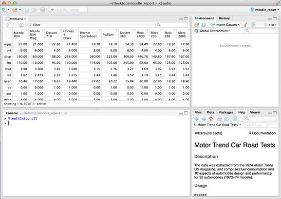
The fundamental difference between data frames and matrices in R is that matrices can only contain a single data type while data frames can have a different data type in each column. The transpose function first converts the data frame to a matrix – so all data is converted to the “least common denominator” data type. This is evident in the mtcars dataset in the gear column.
In the worst case, you end up with a bunch of strings, which is often not intended. This can happen if row names are included as part of your dataset rather than being part of the metadata of the data frame accessible using the rownames function.
More Reshaping of Data
The reshape2 includes two methods (“melt” and “cast“) to change the form, but not the content of a data frame. The base R language can perform comparable transformations, but uses a number of different functions and operators that are not particularly unified or consistent. The reshape2 package provides a streamlined and consistent syntax for these operations.
Before we begin, we will manipulate row names using the inverse of the operation shown earlier. Rather than pulling a column out of the dataset and assigning the column values as row names, the row names will be included inline in the dataset.
|
1 2 |
df<-mtcars df$car_name <- rownames(mtcars) |
The melt function takes each column and represents the data by creating a column to hold the (old) column name and a second column to hold the actual value. Any columns listed in the id vector are retained.
|
1 |
melt(df, id="c(""car_name")) |
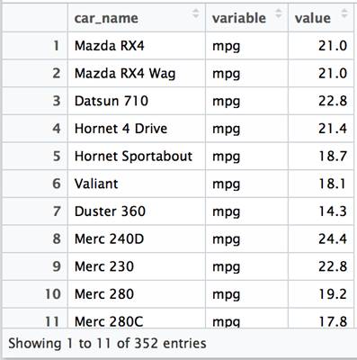
The variable column contains entries for each column in the original dataset (mpg, cyl, disp, hp, etc). A row is created for each value associated. This presents the data in a “long” rather than a “wide” format.
The default version of the function selects an id column to use based on data types available (and works as expected with df). When called in this manner, all columns with numeric values are treated as variables with values and the car_name column is assumed to be an id column. So the results are the same as those shown above.
|
1 |
melt(df) |
This function selects the “name” column by default with the current dataset. In this example, we named the column car_name as it is more explicit, and it prevents problems with other functions that treat columns named “name” in a special way.
Just to emphasize, this is not the only way to use the melt function, and different results are possible by modifying the call to this function. The following example retains the gear data in a column along with the name column as previously shown.
|
1 |
melt(df, id="c(""car_name","gear")) |
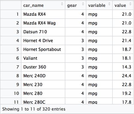
The gear column is not included as a value in the variable data, but instead is retained as a column. As a result, the total number of rows in the dataset is reduced. The data is a bit “wider” than the previous example, but it is not a particularly practical arrangement.
We will store the melted data in a second data frame.
|
1 |
melted <- melt(df, id="c(""car_name")) |
The complementary function for melt is cast. There are a few variations on this function that allow you to choose what data structure is returned. We will use the dcast variation that returns results as a data frame. We will store the results in a variable and will look at them a bit closer in the next section.
|
1 |
df2 <- dcast(melted, car_name ~ variable, value.var = c("value")) |
The tilde ~ operator is typically used in R to separate the left and right hand sides of a formula. While the data has been converted back and forth without changing the content of the data, the row and column order may have changed.
At this point we have two data sets, the original, and a second dataset that has been melted and recast. To do a final comparison that demonstrates these are identical, we need to perform a few operations that order the columns and rows. If we don’t perform these steps, the two data frames will be considered “not equal” simply because the rows or columns are ordered differently. These steps essentially “normalize” the datasets by sorting the columns and rows in alphabetical order by row name.
The row names is stored in alphabetical order in a vector.
|
1 |
cn <- sort(colnames(df)) |
Two new dataframes are created containing the data with the columns in alphabetical order.
|
1 2 |
original<- df[cn] reshaped<- df2[cn] |
The data itself is reordered so that rows are in alphabetical order by name.
|
1 2 |
original <- original[order(original$car_name),] reshaped <- reshaped[order(reshaped$car_name),] |
Because rownames are metadata and we have included them as the names column in the data frames, we will not consider them in the comparison of the two data frames.
|
1 2 |
rownames(reshaped)<-NULL rownames(original)<-NULL |
With these arrangements in place, the original dataset and the melted-recast dataset contain the same data.
|
1 |
all.equal(original, reshaped) |
The function call returns TRUE, indicating that the two data frames contain identical values. If you wanted to retain this set of transformations for use in subsequent tests, you can use the following function.
|
1 2 3 4 5 6 7 |
normalize_df <- function(df, sort_column){ cn <- sort(colnames(df)) df <- df[cn] df <- df[order(df[sort_column]),] rownames(df) <- NULL return(df) } |
This function can compare the data frames without the need to run each normalization step manually.
|
1 2 3 4 |
all.equal( normalize_df(df, 'car_name'), normalize_df(df2, 'car_name') ) |
R lends itself to simple interactive examples. Functions like this suggest one of the most useful techniques to learn the R language. In a few lines of code, a function of this sort can be created to verify an operation is behaving as expected. Often the best way to ensure you understand what R is doing is to create simple examples to test and validate your expectations.
Reshaping and Tidy Data
Programming languages can be classified by basic philosophy that drives the design of the language and impact subsequent community activity such as package development. TIMTOWTDI (pronounced “Tim Toady”) stands for “There is more than one way to do it” and was popularized by the Perl community. While some programmers appreciate the flexibility afforded by such an approach, others are irritated by the ambiguity introduced. Languages like Python take the opposite approach and are designed so that there is only one way to do things whenever possible. Regardless of your opinion on the best approach, it is important to realize that R packages have significant overlap in terms of functionality. Often features available in the base language are packaged as a domain specific language in a particular package for consistency or convenience. An awareness of this fact will prevent confusion and make you more effective at selecting packages to rapidly solve problems.
The tidyr package includes functionality found in the reshape2 package but the overall design has a different purpose. Load up the package to see the similarities demonstrated below.
|
1 |
library(tidyr) |
The tidyr package contains methods that correspond to melt and cast: gather and spread. The gather function is called along with the “bare” column name – the name of the column without enclosing it in quotes.
|
1 |
melted_tidyr <- gather(df, car_name) |
The only difference between the dataframe in this case with the one produced by reshape2 is the rownames. The all.equal method includes an option to ignore the rownames.
|
1 |
all.equal(melted, melted_tidyr, check.names=FALSE) |
The function call returns TRUE. We will ensure that the column names are unique by explicitly naming them and then call the spread function to convert the data back to its original format.
|
1 2 |
colnames(melted_tidyr ) <- c('car_name', 'variable', 'value') spread_tidyr <- spread(melted_tidyr, variable, value) |
The final result is a data frame that matches the original (once the data frames are normalized).
|
1 2 3 4 |
all.equal( normalize_df(df, 'car_name'), normalize_df(spread_tidyr, 'car_name') ) |
The reshape2 package is designed for general purpose reshaping of data. The tidyr package is specifically designed for getting data into a “tidy” format. Hadley Wickham coined the term “Tidy Data” and is the author of the packages referenced in this article. It is a standardized form for data – closely related to the idea of normal forms in databases – that simplifies subsequent analysis and processing.
SQL-like Manipulations in a Functional Style
SQL is the standard language for manipulating data in relational databases and has influenced a variety of query languages in non-relational data stores. It can be used to manipulate data frames in R using the sqldf package. The dplyr package provides functions comparable to those available in SQL.
|
SQL Keyword |
dplyr |
|
SELECT |
select, mutate |
|
WHERE |
filter |
|
ORDER BY |
arrange |
|
GROUP BY |
group_by |
|
HAVING |
filter |
Besides its practical usefulness, the package is interesting as it provides a different way of constructing data manipulation that is based on functional programming and pipes rather than SQL statements. The value of this approach becomes more apparent when long complex queries consisting of nested subqueries are replaced with a chain of piped functions.
The dplyr package was introduced in the R-Basics post. The dplyr library uses the operator (%>%) to stream the results of one function to the next (like UNIX pipes). This operator is available as soon as the library is loaded and can be used with functions that are not part of dplyr itself.
|
1 |
library(dplyr) |
SELECT
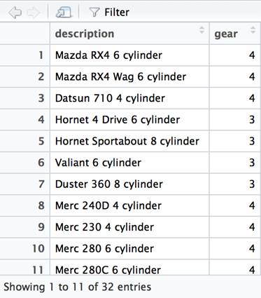
The functions that correspond to the SQL SELECT statement are select() and mutate(). We will use a piping operator to chain together calls on the data frame based on the mtcars data frame. The mutate column is used to add derived data frame columns. In this case, we will append the car name, the number of cylinders and the string literal cylinder. This new column will be named description. We then filter which columns will be viewable and restrict them to the new description column and the gear column. Finally, we will pipe to the View function (which is not part of dplyr) which will display the final result.
|
1 2 3 4 5 |
df %>% mutate(description=paste(car_name, cyl, 'cylinder')) %>% select(description, gear) %>% View() |
ORDER BY
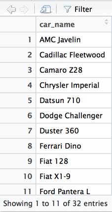
The ORDER BY function is used to sort the data based on one or more columns. The arrange function is the dplyr equivalent.
|
1 |
df %>% select(car_name) %>% arrange(car_name) %>% View() |
GROUP BY
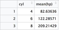
The SQL GROUP BY clause is used in close conjunction with aggregate functions like SUM() and MEAN(). The clause indicates the level of grouping at which a given summary function is applied. When using the dplyr package, it is common practice to use the summarize and group_by functions together.
|
1 |
df %>% group_by(cyl) %>% summarize(mean(hp)) %>% View() |
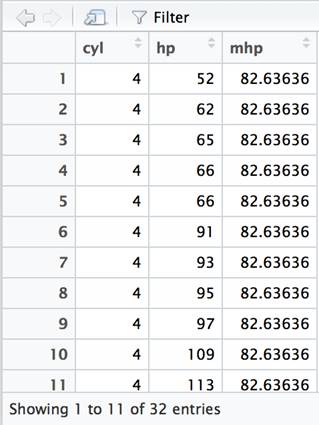
In SQL, it is necessary to list the columns referenced in the GROUP BY clause in the SELECT clause – along with any aggregate functions. The dplyr package just requires you to specify the function used to aggregate in the summarize clause. The dplyr functions can be chained together in creative ways that would require nested subqueries in SQL. For instance, if you wanted to compare the average just calculated with the actual value in each row, this can be accomplished using the mutate function rather than summarize.
|
1 2 3 4 |
df %>% group_by(cyl) %>% mutate(mhp=mean(hp)) %>% select(cyl, hp, mhp) %>% arrange(cyl, hp) %>% View() |
WHERE/HAVING
The WHERE clause in SQL is used to filter which rows are returned. The HAVING clause is used when evaluating summaries that rely upon a GROUP BY. The simplest case is filtering using an equality operator.
|
1 |
df %>% filter(car_name=='Volvo 142E') %>% View() |
![]()
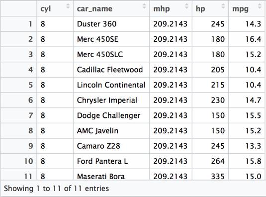
This example is essentially the same usage that you would obtain using a WHERE clause in SQL. The next example uses an aggregate function inside of a filter function. This corresponds with the SQL HAVING clause. Note that the results include records which have an actual horse power (hp) that is less than 200. However, they are part of the grouping (by cyl) that is greater than 200.
|
1 2 3 4 5 6 |
df %>% group_by(cyl) %>% mutate(mhp=mean(hp)) %>% filter(mhp > 200 & mpg < 17) %>% select(car_name, mhp, hp, mpg) %>% View() |
As this example illustrates, the arrangement of functions in a chain is less restrictive than the structure of SQL queries. Each function is independent and discrete, whereas a unit of work in SQL is a statement that must contain a SELECT and may contain the other clauses referenced. SQL statements can be nested using subqueries to effectively “chain” together SQL statements. The dplyr function interface is less verbose and more focused on the specific aspects of the data that are changing with each step processed.
R a Data Manipulation Platform
SQL is – by definition – a query language. It excels at retrieving data from a database and is in fact essential in many situations where it is the only way to get data out of a database.
However, SQL can be cumbersome when it is used to transform data. SQL is very flexible and so does support the ability to transform data in significant ways, but often with the cost of requiring verbose, obscure, and difficult to support SQL statements. R includes a number of packages that can perform such operations in a concise, clear, simple manner. It is well worth the time to learn these packages so that the best aspects of both SQL and R packages can be used to analyze data using a series of steps that is easy to understand and comprehend.
Load comments