When Microsoft introduced table partitioning in SQL Server 2005, we welcomed the ability to switch partitions to or from a table, allowing us to implement data import with minimum locking. We can use partitioning to purge millions of records in a matter of milliseconds and, more recently, to update tables with ColumnStore indexes, which are technically read-only. Finally, partition elimination can sometimes help with query performance.

Unfortunately, there is no such thing as a free lunch. Partitioning changes how data is physically stored, and often leads to additional storage space requirements. More significantly, perhaps, it can also mean changes to the execution plans, often resulting in sub-optimal plans and poor performance.

In this article, I’ll explain why we need to be aware of these two issues when we partition our data, and suggest workarounds.

Storage space increase

A key design consideration, when planning for partitioning, is deciding on the column on which to partition the data. SQL Server requires the partitioning column to be part of the key for the clustered index (for non-unique clustered indexes, if we don’t specify the partitioning column as part of the key, SQL Server adds it to the key by default). For unique clustered indexes the partitioning column will ideally already be part of the clustered index but often it’s not, unfortunately. The common solution, in that case, would be to add the partition column as the right-most column of the clustered index.

Storage requirements for the clustered index would not change much since the column data is already at the leaf level. It would increase the size of the record at non-leaf levels though and, in some edge cases, could even introduce another level to the index. Fortunately, this rarely happens unless the partition column is very wide, but if it does then we will have an extra logical read for every key lookup operation against the table.

However, storage space for non-clustered indexes would increase. A non-clustered index uses the clustered index key value as the record pointer. Partitioned tables are usually large and by adding a new column to the clustered index key, we increase the record size in every non-clustered index on the table. For example, let’s say we add an 8-byte datetime column to the clustered index key, for a table with 500,000,000 rows (frankly, not that huge a number, these days). We will end up with 500,000,000 * 8 / 1,024 / 1,024 / 1,024 = ~3.72GB of storage space per index just to store value itself. This figure does not include storage space at non-leaf levels and storage overhead produced by fragmentation. In turn, this will increase the size of database backups as well as restore times, and will increase the index maintenance cost.

Unfortunately, this can sometimes create problems for which there aren’t easy solutions. Let’s say that the business requirement is for the system to keep data in the table for twelve months, and at the beginning of each month to purge data for the thirteenth month. These requirements also state that the table must remain online during the purge process and that it shouldn’t cause excessive blocking of user operations. While these requirements don’t dictate the technical solution, they certainly point strongly towards use of the “Sliding Window” pattern, partitioning the table on the date column. One alternative option might be to delete data in the smaller batches, although purging via the partition switch would be much more efficient and less transaction log intensive operation.

However, suppose the most recent 12 months’ data is stored on our fastest storage tier, on which there is limited space. Sometimes we can be creative, but none of the alternatives to adding the date column to the clustered index is straightforward.

For example, if we have a table with an IDENTITY column, which is part of the clustered key, we can use that column rather than the date column. Be careful though, as this opens its own assortment of problems: SQL Server would not be able to perform partition elimination, unless we refactor the queries. If we partition by date and query for a specific month then SQL Server would only need to access the partition containing that month. In other words, it can exclude, or eliminate, from the processing any partitions where it knows that the required data cannot exist. Unfortunately, this would not work in the approach with IDENTITYcolumn, unless we look up the ID values belonging to particular month (partition) and add them to the query as additional filters.

Another possibility might be to create a non-unique clustered index on the date column and make the existing clustered index non-clustered.

Whichever solution we choose, we need to analyze how partitioning would affect the system not only from a storage standpoint, but also in terms of performance.

Suboptimal execution plans

When we implement table partitioning, we change the physical data layout and this, in turn, can result in different execution plans for our queries, and sometimes those changes are quite unexpected. Let’s look at an example.

Consider a process that polls a table, based on some time interval, and selects a batch of the recently modified records. We might see this sort of implementation in a process that performs data synchronization between two different databases and/or vendors, or in a data processing framework, that loads the data. Obviously, there are several ways to accomplish this task with out-of-the-box SQL Server technologies. This example will be a simple T-SQL implementation.

Listing 1 shows the structure of the Orders table, with clustered index.

Listing 1: The Orders table structure

The OrderDate column stores the time the customer placed the order. The DateModified column records the last time someone modified the order. The Placeholder column can be assumed to be a simplified substitute for several columns that would store any additional information, or special instructions, regarding an order in a real system.

Listing 2 inserts 524,288 records into the Orders table and creates a non-clustered index.

Listing 2: Test data insert

Note that in this example we assume that we cannot add Placeholder to the non-clustered index, as an included column, due to its size. This means a Key Lookup will be necessary for any query that returns this column.

The process that reads the data from the table uses a @LastDateModified parameter, populated based on the last record from the previous batch read, as shown in Listing 3.

Listing 3: Query that selects the batch of the records

For the sake of simplicity, we’re ignoring for now a few problems with such an implementation, which can result in SQL Server not selecting some records, for example if DateModified is not unique, or when concurrency and blocking are involved.

Let’s run the query in Listing 3, against our un-partitioned Orders table, and examine the execution plan and statistics IO, as shown in Figure 1.

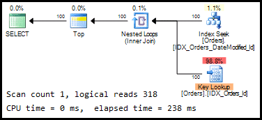
Figure 1: Execution plan for un-partitioned Orders table

The plan is as efficient as it could be, in the circumstances described. We have an ordered index seek for the non-clustered index, plus a key lookup on the clustered index for each of the rows. It makes a lot of sense if we think about what is happening under the hood, as depicted in Figure 2.

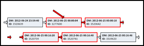
Figure 2: Leaf level of the un-partitioned non-clustered index

When we run the query, SQL Server locates the first record that has a DateModified value greater than the value of @LastDateModified, and retrieves the next 100 records from that point onwards. The order of the data in the index matches the ORDER BY clause, so no further sort is required. This is a simple and relatively efficient approach.

What will happen, however, if we partition our Orders table? For such a table, the natural candidate for the partitioning column is OrderDate. In Listing 4, we drop our two indexes, create the partition function and scheme (partitioning on a monthly basis), and then recreate the indexes.

Listing 4: Table partitioning code

Notice that we have aligned our non-clustered index with the partitioned table. We could have kept it un-aligned, but that would prevent us from using partition switching and has other implications. Having aligned the index, its physical data layout has changed, as shown in Figure 3.

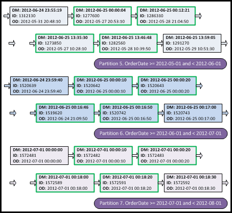
Figure 3: Leaf level of partitioned non-clustered index

As we can see, our index consists of the multiple physical partitions. We can think about them almost as if they were separate tables. The key point is that data is sorted only within the single partition and this means that our current execution plan (Figure 1) is no longer valid.

How do we envision the “ideal” execution plan for our query against the partitioned table? Given that the data within each partition is sorted, the first step, illustrated in Figure 4, is to select 100 records from each partition.

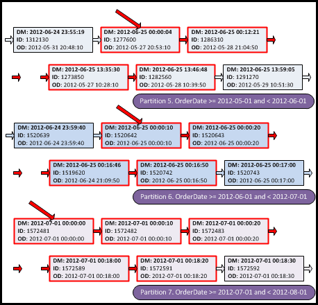
Figure 4: “Ideal execution plan”. Step 1: select 100 records from each partition

The next step is to sort the selected records from Step 1 and select the first 100 records from that sorted record set, as shown in Figure 5.

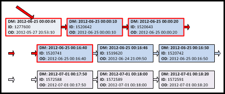
Figure 5: “Ideal execution plan” – Step 2: Top N Sort of selected records

The cost of the plan would depend on the number of partitions in the table. It would not be as efficient as the plan for the un-partitioned table, but it should still be acceptable.

Figure 6 shows how SQL Server actually processes the query.

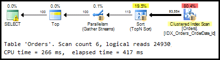
Figure 6: Actual execution plan for Listing 3, using the partitioned table

This time, the optimizer ignores our non-clustered index and simply scans the clustered index. As you can imagine, this could be very an unpleasant surprise when we push the changes to production.

Perhaps we can force SQL Server to use non-clustered index with an index hint.

Listing 5: Select with index hint

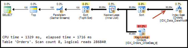
Figure 7: Actual execution plan with index hint

Even if that plan looks close to what we were hoping to see, it’s not the same. SQL Server does not stop after it selects 100 records from each partition. Instead, on each partition, SQL Server starts from the first record with DateModified that has a value greater than @LastDateModified, and the scans the index to the end of partition. In our example, SQL it selected 93,554 rows and performed key lookups for all of them when, in fact, it should be selecting 800 records at most (up to 100 records from 8 partitions). This plan might still be acceptable when there is no backlog involved, and we have very small number of records where the DateModified value is greater than @LastDateModified. However, generally speaking, this approach is unpredictable.

In cases where it’s not possible to make the index covering, there is no easy way around this problem. Even if the query optimizer does a great job most part of the time, there is always the possibility that table partitioning will negatively affect the performance of some queries. The only method that helps is testing. Fortunately, it’s not very hard to pinpoint affected queries as long as test coverage is good enough, and then we need to refactor the problem queries, one by one.

Fixing the problem

There is no silver-bullet solution here, which will work for every query, but in most cases, the solution is to perform some kind of manual partition elimination, meaning that we try to force SQL Server to deal only with specific partitions. When SQL Server queries the data from within the single partition, the resulting plan, as shown in Listing 6, is almost identical to the one obtained for the query against the un-partitioned Orders table.

Listing 6: Execution plan when selecting data from the single partition

We’ve used the function, $Partition, which returns the partition number for the arguments provided. By adding it to the WHERE clause of the query, we’ve forced SQL Server to deal with a specific partition only.

If we could extend this behavior to the entire table, rather than just a single partition we’d have something close to our “ideal” plan (as expressed in Figures 4 and 5).

In order to do this we first need to know the number of partitions in our table. There are a few ways to get this information through the data management views. Here, we’ll use the sys.partition_range_values view to return the boundary values for the partition function. By adding one to the number of boundary values, we get the total number of partitions in the table.

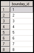
Listing 7: Getting list of boundary_id values for the partition function

Now we can force SQL Server to run 8 individual selects, each on an individual partition, by using CROSS APPLY with a filter condition of $Partition.pfData(DateCreated) = boundary_id. This implements step 1 of the “ideal” execution plan we defined earlier in Figure 4.

Listing 8: Implementation of Step 1 of “Ideal execution plan”

Figure 8 shows the result set we get for Listing 8, including partition number. At most, we can have 800 rows (eight partitions up to 100 records each). We got 300 records only because in the first five partitions there is no data with with DateModified value greater than @LastDateModified.

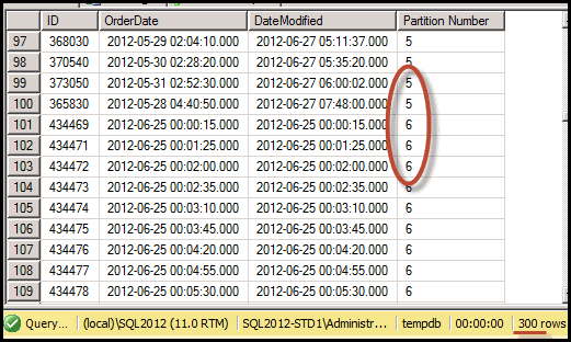
Figure 8: Step 1 of “Ideal execution plan” – results

Figure 9 shows the execution plan for Listing 8. It looks a little complex due to the Boundaries CTE (green area of the plan), although it does not contribute much to the plan cost.

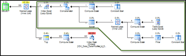
Figure 9: Step 1 of “Ideal execution plan” – execution plan

A couple of other points are worthy of note. First, at this intermediate stage, our non-clustered index covers the query and there are no key lookups. Second, and more importantly, SQL Server stops after it selects 100 records per partition. It no longer scans and sorts the remaining data in each partition, as it did when we used the index hint in Listing 5.

Next, we need to sort the data we got in the previous step and return the top 100 records. The final version of the code would look as shown in Listing 9.

Listing 9: Final version of code to achieve “ideal” execution plan

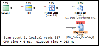
In the Top100 CTE, we sort the records and return the 100 we need. Our non-clustered index is still covering that part of the query. In the outer SELECT, we join the data from non-clustered with that from the clustered index, essentially emulating a regular key lookup operation. By moving the join to the outer select, we reduce the number of “lookups” to the number of records in the final resultset. Figure 10 shows the execution plan.

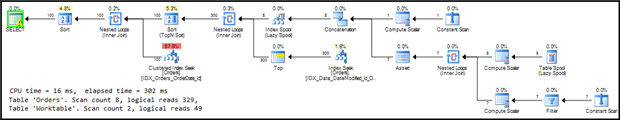
Figure 10: Final execution plan

As we can see, it’s almost as perfect as it could be in that from each partition we select only records that can potentially be in the final resultset. SQL Server performs the sort against those records only and, finally, accesses the clustered index only for the data we need.

Dealing with Cardinality Estimation Errors

One of the downsides of such an approach is cardinality estimation errors. SQL Server is unable to estimate the number of records returned by the Boundaries CTE and, as result, the number of CROSS APPLY executions. It assumes that the Boundaries CTE returns only two records. The under-estimation error would propagate up to the Sort operation in the outer select of the Top100 CTE and could potentially lead to a memory grant that was too low, and a subsequent spill to tempdb, especially with a large number of partitions and a lot of data. When SQL Server has to use tempdbinstead of memory for sort and hash operations, it can degrade performance dramatically. There are a few ways to detect the problem, such as by monitoring Hash and Sort Warnings events in SQL Profiler, In SQL Server 2012, query plans also displa y these warnings and we can capture them with extended events.

We’ll consider two ways to improve the cardinality estimation, first by using temporary table instead of the CTE, and second by hardcoding the number of partitions into the CTE. Neither solution is perfect. The first is susceptible to cardinality overestimation, rather than underestimation, and the second requires us to change our queries if we ever change the number of partitions in our table, so is harder to maintain.

Using a Temporary Table instead of CTE and recursion

We can solve this by using a temporary table to store the boundary_id values, rather than using recursion in the Boundaries CTE. SQL Server will keep statistics on the temporary table primary key, and would be able to estimate the number of execution correctly.

Listing 10: Using a temporary table in order to improve cardinality estimation

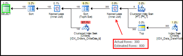
Figure 11: Using temporary table in order to improve cardinality estimation

However, this approach could lead to over- rather than under-estimation of the number in the records, in cases where some partitions don’t have data. This could lead to an overestimated memory grant and so a query that consumes more memory than it actually needs. It could also lead to unnecessary memory grant waits.

Hardcoding the number of Partitions

Listing 11 shows an alternative way to deal with cardinality estimation errors, by hardcoding the number of partitions in the Boundaries CTE. This is a valid approach as long as this number is static. For example if we have one years’ worth of data in the partitioned table and implement the sliding window pattern to remove data on a monthly basis then the number of partitions in the table will stay the same.

Listing 11: Hardcode static number of partitions in order to improve cardinality estimation

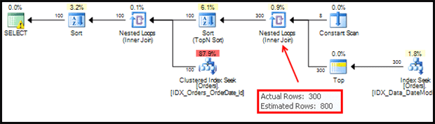
Figure 12: Hardcode static number of partitions in order to improve cardinality estimation

As noted earlier, if we ever change the number of partitions in our table then we’ll have to rewrite our query in Listing 11.

Summary

While table partitioning is a great feature that can help with various design and performance challenges, it could also create its own set of problems. Adding partitioning column to non-clustered indexes increases the storage space and index maintenance cost. Different physical data layout changes execution plans for the queries, which in some cases can negatively affect performance. It’s extremely important to know about those side effects and test the system before applying the changes in production.