In my last article, I explained how the Date_Correlation_Optimization works, and demonstrated that we can achieve considerable performance gains in our queries if we use it properly. This time round, we’ll see a deeper analysis of this feature, and we’ll look under the hood to see how it works and what logic the Query Optimizer used to identify the correlation between the two datetime columns. The first question what we need to answer is:

What does SQL Server do to discover the values used as a filter in the query? (specifically as a filter for the Data_Entrega column)

So, let’s get started!

The code generated by Query Optimizer

If you recall, In my last article I said that “SQL Server gets the information about the correlated columns and keeps this information to use as SQL Statistics“. To be more specific, the SQL Server creates an indexed view with the information about the correlated columns.

To start with, we’ll create the sample metadata structure presented in the first article, but this time we’ll execute the script in discrete blocks so that we can observe the code being generated by SQL Server. Go to SQL Server Management Studio and execute the necessary script, but just the part for the creation of the tables and the clustered index.

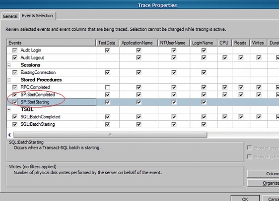
After creating the tables and adding the clustered index to the Items table, let’s configure a trace to capture some data about the code being generated by SQL Server to create and manage the indexed view we’re interested in. Open the Profiler, create a new trace, and select the SP: StmtCompleted and SP: StmtStarted events, as they will show us the code we want to know more about.

After starting the trace, execute this code…

… and the Profiler Trace will capture the following rows:

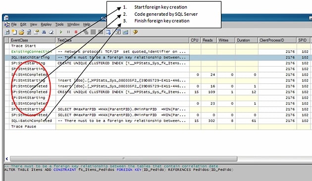
To be more precise, here is the code:

As we can see, the SQL Server has generated three commands; the first one adds an index to a view called _MPStats, the second inserts data into that view and third SELECTs using that view. Before we do anything else with this data, we need to understand where this view has come from…

Understanding the view created by SQL Server

The profiler trace cannot show us the code with the newly-created view, but using a select at sys.views, we can see that it was definitely created internally by SQL Server.

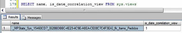
Notice the is_data_correlation_view column, which tells us that this view is used by date correlation. At first glance, the name of this view is a little odd, but there is a logic behind it:

_MPStats_Sys_<constraint_object_id>_<GUID>_<FK_constraint_name>

Using that rule, we have the following name:

_MPStats_Sys_15460CD7_{628BDBBC-4E23-4C9E-A8EA-CE08C7C4F3EA}_fk_Items_Pedidos
 
Where:

• Violet – Fixed value.
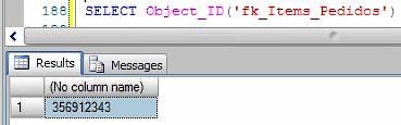
• Red – The hexadecimal Foreign Key Object_ID. Just FYI, if you want to be sure about whether this value is correct (like me), you could transform the it into a decimal and check if this value corresponds to the name used by SQL Server. For instance:

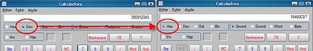
• Green – GUID generated internally by SQL Server.
• Blue – Name of the foreign key linking the tables.

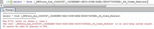
If you try to do a SELECT using that view to see what it returns, you’ll receive the following message:

To make this SELECT work and show you the data stored in the view, you’ll need to create another view based on the system view. The question which pops up here is, obviously, “What can I do to know the code of this view?” Easy, just run the sp_helptext:

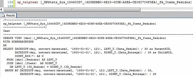
Don’t worry about this code for now, we will study it and see what that means soon. But now that we have the code, let’s go and create another view called vw_test.

Now we can make the SELECT work, but the Pedidos and Items tables are currently empty, so let’s go and insert some data.

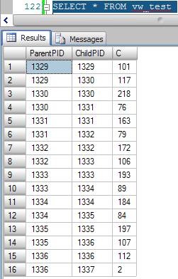
No we’ll make a SELECT into vw_test to see what data it contains. Remember, we have created the vw_tests to see what data is stored in the view created internally by SQL Server. The code of both is the same, so we have an exact replica of what is saved in the original view.

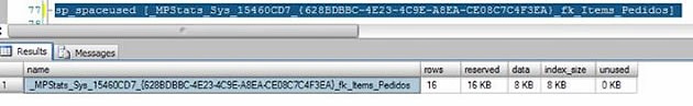
It’s important to bear in mind the fact that is an indexed view; in other words, it uses a fair amount of disk space and needs to keep being updated whenever INSERTs, UPDATEs and DELETEs occur in the Pedidos and Items tables. So, if you notice that the writing events to your table are taking a long time to run, you should check if this view is causing the problem. If you want to see how much space the view is using, run the proc sp_spaceused.

Understanding the Magic

Now that we’ve understood when the view is created and how it is used, let’s try to understand the more important step: What is the logic used to identify the values of the correlated columns?

In the view we have two columns, ParentPID and ChildPID. The following rule is used to return the values of these columns.

Translation:

SQL Server, for ParentPID and ChildPID, I want to you return how many days I need to go from 1900-01-01 until I reach the date stored in the Data_Pedido column, then divide this value 30. For instance: To go from 1900-01-01 until 2009-01-01 we need 39812 days, and dividing this values by 30 we have 1327.

The SQL Server divides these days’ values by 30 to keep the aggregated data lower. Naturally, if the divisor is bigger ,the result of the aggregation will be lower, and if the divisor is lower the result of the aggregation will be large – Thirty is a good number to use because it’s close to a month.

When we build a query using the Data_Pedido column, SQL Server get the values which we have used in the WHERE clause and applies the same formula as above to get the number of days divided by thirty. The Query Optimizer goes to the view and searches for the value of ChildPID(Data_Entrega) using a filter for the value of PartentPID (Data_Pedido), which is the value just calculated. When it finds the ChildPID value, it applies the same formula again, but in the opposite direction to get the value that will be used as a predicate in the Items table filter.

Ok, I know that, reading this, it seems to be a little confusing. Let’s go see that in practice and step by step it will become easy to understand. Suppose we have the following query:

As we can see, there is a filter applied to the Data_Pedido column, and the SQL needs to know what values we will use as a predicate to filter the Items table too. Let’s go step by step, now:

• The Query Optimizer goes to the view to identify what are the max and min values of the ChildPID column to make the reverse calculation. You can see this query (generated internally by SQL Server) using the profiler trace.
  • Thefollowing query was executed, I’ve changed t  a little for readability, but you will capture code very similar to this in the profiler trace.

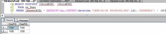
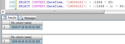
• With the values 1334(min) and 1335(max) in hands the SQL, it applies the inverse rule to get the values that will be used to filter the Data_Entrega column.

Translating:

From the date 1900-01-01 to (1334 * 30), (in this case) we have 2009-07-28 as the min value. To get the max value, the SQL Server adds 1 to the max read value in the view (In this case 1335 + 1). In my honest opinion, it uses this to be sure about not changing the result set.

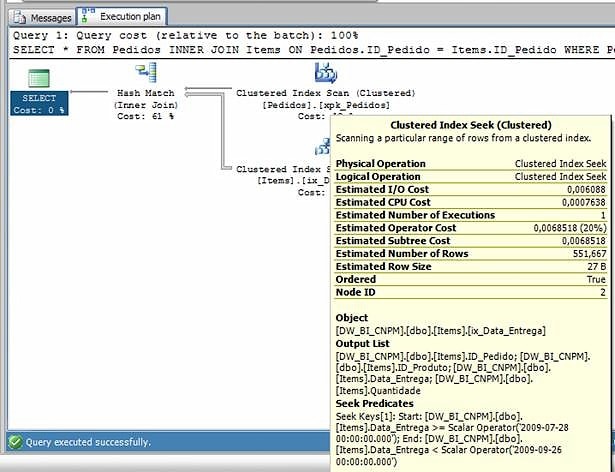
• SQL Server uses the data values as a filter for the Items table. Looking at the execution plan, we can see that it was using the exact values that we got in step 2:

Summary

So, we’ve seen under the hood of how that feature works, and you may have learned some other tricks like capturing the queries generated by SQL Server, converting values from hexa to decimal, sp_helptext, sp_spaceused etc. I want to get one thing clear, though; for the time being I’m not a SQL product developer, so I may be wrong in some of the finer details of what I’ve just presented. I’ve not confirmed with the SQL developer team if my logic is 100% correct, but if you understood my reasoning you will see that it makes complete sense.

To finish I want to leave you with an interesting thought. The same logic presented above can be used in a lot of other situations, yes? I think it is worthwhile spending  a little time thinking about it. I hope you’ve enjoyed these two articles; all feedback is appreciated, so please feel free to leave some comments below.

That’s all folks.