Sometimes, solutions to the simplest sounding requests can be very difficult to implement. A case in point is Phil Factor’s second Speed Phreak Competition: The ‘FIFO Stock Inventory’ SQL Problem. The competition presented a somewhat-simplified, but still realistic inventory accounting problem, where approximately 1500 different stock items are either purchased, sold, or returned. The mission was to calculate the remaining count, and value, of each item after all stock transactions are performed, using only T-SQL. This is a classic FIFO (First In, First Out) problem, or a queue, where the first items purchased or returned must be the first items sold.
In my previous article, based around the Running Total Speed Phreak challenge, I commented that, in my experience, there is usually “an easy solution and a fast solution”. The easy solution, often iterative and cursor-based, is simple to implement, easy to maintain, and straightforward. However, performance often becomes painfully unacceptable as the volume of data grows. The fast solution, usually set-based, is often harder to understand, and therefore maintain, but will perform well and scale gracefully.
The motivation behind this series of articles was to dissect and analyze the cleverest and fastest SQL solutions to the challenges posed by the Speed Phreak competitions, expose and explain the core set-based techniques on which they rely, and so make these techniques more widely accessible to developers who need a faster and more scalable solution than the cursor can offer.
This FIFO challenge is considerably more complex that the previous Running Total challenge, and my motto, “there’s an easy way and a fast way”, doesn’t quite hold true. Here, it turns out that there’s a “slow and difficult” way, using a cursor, and a “fast and even more difficult” way, using set-based techniques. This time it helps to not only think outside the box but to turn the box inside out.
The FIFO Stock Inventory Challenge
In this challenge, we have a table, Stock, which we use to track the track movements of stock in and out of our imaginary stock warehouse. Our warehouse is initially empty, and stock then moves into the warehouse as a result of a stock purchase (tranCode = ‘IN’), or due to a subsequent return (tranCode = ‘RET’), and stock moves out of the warehouse when it is sold (tranCode = ‘OUT’). Each type of stock tem is indentified by an ArticleID. Each movement of stock in or out of the warehouse, due to a purchase, sale or return of a given item, results in a row being added to the Stock table, uniquely identified by the value in the StockID identity column, and describing how many items were added or removed, the price for purchases, the date of the transaction, and so on.
Stock movements always occur on a first-in, first-out (FIFO) basis, so the stock initially purchased or returned is the stock that is first to be sold, and the current stock inventory for a given ArticleID will consist of those items that were the last to be added to the inventory. The challenge, in essence, was to find the most efficient way to calculate the value of the remaining stock for a given item, given that:
- There is a price for each purchase
- Items are sold in the order that they were purchased or returned
- The price of each item sold is based the price based on when the item was acquired
- Each return should be priced at the same price as the most recent purchase before the return
Included with the challenge description was an abbreviated example, as follows in Table 1:
|
StockID |
ArticleID |
TranDate |
TranCode |
Items |
Price |
CurrentItems |
CurrentValue |
|
4567 |
10000 |
10:45:07 |
IN |
738 |
245.94 |
738 |
181,503.72 |
|
21628 |
10000 |
12:05:25 |
OUT |
600 |
138 |
33,939.72 |
|
|
22571 |
10000 |
14:39:27 |
IN |
62 |
199.95 |
200 |
46,336.62 |
|
30263 |
10000 |
16:14:13 |
OUT |
165 |
35 |
6,998.25 |
|
|
42090 |
10000 |
18:18:58 |
RET |
5 |
40 |
7,998.00 |
|
|
53143 |
10000 |
20:18:54 |
IN |
500 |
135.91 |
540 |
75,953.00 |
Table 1: Example of stock movement
- First we add 738 items (each $245.94) to the stock, for a total of $181,503.72
- Then we take out 600 items (each 245.94) from the stock, leaving a total of $33,939.72
- Then we insert 62 items (each 199.95) to the stock, for a total of $46,336.62
- Then we take out 165 items (138 each 245.94 and 27 each 199.95), leaving a total of $6,998.25
- Then we return 5 items. We can’t track at which price we took them out; so all returns are priced at the price of the latest ones inserted before the return. Even if there should be items left for the price of 245.94, the returned items are valued for 199.95. After the return, the current stock value is $7,998.00
- The final purchase (each $135.91) adds $67,995.00 to the stock value, for a total of $75,953.00
A sample cursor solution was provided with the original challenge and entrants were asked to come up with something better, given the following rules:
- Calculate the number and value of each ArticleID after all the transactions are processed
- The results must be in
ArticleID order You can use any method you prefer as long as it involves only T-SQL You can use a tally, or numbers, table called TallyNumbers, beginning with 0 Running totals are provided in the sample data to help validate your results, but you can’t use them in the solution You cannot alter the design of the Stock table, but you can alter the provided non-clustered indexes The CurrentItems and CurrentValue columns are provided to allow you to validate your algorithms only; you cannot use them in your solution. Once again, several gifted T-SQL developers came up with very fast solutions to the challenge. The winner was Dave Ballantyne (blog | twitter), whose solution processed a million rows in 3 seconds.
Setting Up
To test the winning solution, your SQL Server instance must be running SQL Server 2008. To set up this challenge perform these steps:
- Create a new database on a development or test SQL Server 2008 instance
- Run the code from Listing 1 to create the Stock table, associated indexes, and the TallyNumbers table.
|
1 2 3 4 5 6 7 8 9 10 11 12 13 14 15 16 17 18 19 20 21 22 23 24 25 26 27 28 29 30 31 32 33 |
CREATE TABLE dbo.Stock ( StockID INT IDENTITY(1, 1) NOT NULL , ArticleID SMALLINT NOT NULL , TranDate DATETIME NOT NULL , TranCode VARCHAR(3) NOT NULL , Items INT NOT NULL , Price MONEY NULL , CONSTRAINT [PK_Stock] PRIMARY KEY CLUSTERED ( StockID ASC ) ) CREATE NONCLUSTERED INDEX IX_Input ON dbo.Stock (TranCode, ArticleID) INCLUDE (TranDate, Items, Price) WHERE TranCode IN ('IN', 'RET') CREATE NONCLUSTERED INDEX IX_Output ON dbo.Stock (TranCode, ArticleID) INCLUDE (TranDate, Items) WHERE TranCode = 'OUT' IF OBJECT_ID('dbo.TallyNumbers') IS NULL BEGIN CREATE TABLE dbo.TallyNumbers ( Number INT NOT NULL ) INSERT INTO dbo.TallyNumbers ( Number ) SELECT TOP ( 1000000 ) ROW_NUMBER() OVER ( ORDER BY A.OBJECT_ID ) - 1 AS Number FROM master.sys.objects AS A CROSS JOIN master.sys.objects AS B CROSS JOIN master.sys.objects AS C CROSS JOIN master.sys.objects AS D END |
Listing 1: The code to create the tables, indexes and helper table
- Download the test data from the http://sql.developerworkshop.net/fifo.zip
- Unzip the file and import the data (consisting of over a million rows) into the Stock table using your method of choice (I used the SQL Server Import Wizard).
Run this query SELECT * FROM Stock to view the data. Figure 1 shows some sample data.
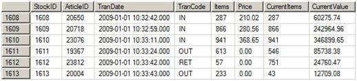
Figure 1: The FIFO data
Remember that you can use the CurrentItems and CurrentValue column values to validate the algorithm, but you can’t just query them to return the answer.
The Cursor Solution
Most of us come to T-SQL initially from a developer background so creating cursor-based solutions is generally easy. With a bit of thought, we often find more efficient set-based solutions without difficulty. This particular puzzle is tricky regardless of which technique you may choose. Because the cursor-based solution may be found along with the original challenge, it will not be reproduced here in its entirety, though is available with the code download bundle for this article (see the downloads at the bottom of the article).
The cursor-based solution calculates the CurrentItems and CurrentValue for each transaction and repopulates those columns in the Stock table. If you set the value of the two columns to zero or NULL in every row of the Stock table, running the cursor-based solution will repopulate the two columns with the correct values. Once completing all the calculations, a query returns the final results.
The code begins by creating a temp table called #work with an Identity column and a column to hold a price. The purpose of the cursor is to populate #work with one row for each individual item received or returned along with the price that applies to that transaction. Because of the Identity column, the rows can easily be sorted in the order in which they were inserted. The items sold are removed from the #work table in order and the remaining rows are used later to calculate the final count of items and the value.
The SELECT statement used for the cursor is ordered by ArticleID and TranDate. Once inside the cursor loop, the code truncates the #work table and resets the @LastPrice variable to NULL whenever the loop processes a new ArticleID. It is very important to the solution to complete all work on one ArticleID before starting on the next.
Each transaction type requires a different action. The extract in Listing 2 shows how the IN and RET rows are processed.
|
1 2 3 4 5 6 7 8 9 10 11 12 13 14 15 16 17 |
IF @TranCode = 'IN' BEGIN INSERT #Work ( Price ) SELECT @Price FROM dbo.TallyNumbers WHERE Number < @Items SET @LatestPrice = @Price END IF @TranCode = 'RET' INSERT #Work ( Price ) SELECT @LatestPrice FROM dbo.TallyNumbers WHERE Number < @Items |
Listing 2: Processing IN and RET rows
If the TranCode = ‘IN’, then a statement inserts rows saving the current price into the #work table. By using the TallyNumbers table, we ensure that the number of rows inserted is equal to the number of items purchased. The @LatestPrice value is set equal to the current price in case it is needed for the next row. If the TranCode = ‘RET’ then several rows are inserted into #work. This is similar to the ‘IN’ transaction, except that it uses the price from the last IN row. Since the #work table contains an identity column (RowID), the order of the inserts can easily be determined.
After processing some IN and RET rows, the #work table will contain one row for each item in stock along with the price for that item. Figure 2 shows an example of how the #work table would look, if you actually stopped the processing to take a look at it, after processing two IN rows that added three items at $258.30 and two items at $260.
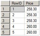
Figure 2: The #work table with some sample data
The next possibility is the movement of items out of stock, or OUT rows. Listing 3 shows the code processes these OUT rows.
|
1 2 3 4 5 6 7 |
IF @TranCode = 'OUT' DELETE w FROM ( SELECT TOP ( @Items ) RowID FROM #Work ORDER BY RowID ) AS w |
Listing 3: Processing the OUT rows
In this case, the code deletes a number of rows from #work equal to the number of items taken out of stock. In order to delete the correct number of rows, the code uses TOP along with the variable @Items. The ability to use a variable along with TOP was introduced with SQL Server 2005 along with the ability to use TOP with a DELETE statement. Unfortunately, you cannot use ORDER BY with a DELETE statement so you can’t guarantee that the correct rows would be deleted. It is critical that the code deletes the rows inserted first, so the deletions are made by using a derived table sorted in the correct order.
After the rows are inserted or deleted from #work, for a particular row from the Stock table, the #work table contains one row for each item remaining in stock for that ArticleID, along the price for each item. The next step is to update the CurrentItems and CurrentValue columns of the stock table for the row currently being processed. Listing 4 shows the section of code used to update Stock. Everything left in the #work table is used to calculate the count and value for the current transaction.
|
1 2 3 4 5 6 7 8 |
UPDATE s SET s.CurrentItems = w.CurrentItems , s.CurrentValue = COALESCE(w.CurrentValue, 0) FROM dbo.Stock AS s INNER JOIN ( SELECT COUNT(*) AS CurrentItems , SUM(Price) AS CurrentValue FROM #Work ) AS w ON s.StockID = @StockID |
Listing 4: Updating the Stock table
The UPDATE statement uses a derived table in the form of an aggregate query that calculates the current number of items multiplied by the current value. The derived table is necessary because you can’t directly use an aggregate query in an UPDATE statement. A common table expression (CTE) could also have been used.
The original data actually contains the correct values for CurrentItems and CurrentValue, and the UPDATE statement overwrites these values. If you set all the CurrentItems and CurrentValue columns to NULL first, the code from Listing 4 sets each row back to the correct values.
Since the cursor-based solution calculated the current stock level and value for every transaction, the answer to the challenge may be found in the row for each ArticleID with the latest TranDate. Listing 5 contains the code to display the final answer.
|
1 2 3 4 5 6 7 8 9 10 11 12 |
SELECT ArticleID , CurrentItems , CurrentValue FROM ( SELECT ArticleID , CurrentItems , CurrentValue , ROW_NUMBER() OVER ( PARTITION BY ArticleID ORDER BY TranDate DESC ) AS recID FROM dbo.Stock ) AS d WHERE recID = 1 ORDER BY ArticleID |
Listing 5: Producing the final answer
This query uses a derived table and the ROW_NUMBER() function to list the rows, along with a row number (recID) for each row. The row numbers are applied in descending order of TranDate, partitioned by ArticleID. This ensures that the last stock transaction for each ArticleID will have a recID value of one. The query is filtered by recID to ensure that only the rows with last tranDate are selected, i.e. those with a recID equal to one. The reason for using a derived table is that you can’t directly filter on the results of the ROW_NUMBER() function. This is another example that would work equally as well with a CTE. Figure 3 shows a sample of the answer.
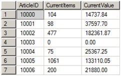
Figure 3: A sample of the answer
This solution performs one update to each row in the Stock table. That’s over 1 million single row updates in addition to either an insertion into, or deletion from, the #work table for each row processed, for a total of 2 million transactions! It does, however, allow you to see the current value at any transaction if you need to do so. The winning solution only calculates the final values for each ArticleID, so it provides much less information. However, if the only requirement is to know the very final values, then this cursor solution is doing much more work than it needs to do.
The Winning Solution
The winning solution, from Dave Ballantyne, takes advantage of many of the new features introduced with SQL Server 2005 and 2008, such as common table expressions (CTEs) and filtered indexes, and manages to solve this problem without a cursor. It returns the answer in an amazing 3 seconds.
Aside from its clever use of use of SQL Server features, it relies on a very important insight into the nature of the problem being solved. The previous cursor solution kept track of the running total, one transaction at a time, as items were added and removed. David realized that in a FIFO problem, this is not necessary: we just need to focus on what is left after all processing is complete.
In order to understand why his is true, let’s consider the age-old practice of emptying our pockets of loose change, at the end of each day, into a “money jar”, but instead of a simple jar we add our coins to a money “queue”, and that we only we removed coins from the front of the queue, meaning that the first coins added are the first coins removed.
Thanks to Dave Mclear for reuse of this photo
If we wanted to calculate the value of the remaining coins on any particular day, would we be concerned about the value of the coins that had already been removed from the front of the queue? Would we have to work through all the additions and removals of coins that had happened over time? No, we could easily calculate the current value just by looking at the remaining coins in the queue.
For example, say I start out by adding a nickel (worth 5 cents each), two pennies (worth 1 cent each) and five dimes (worth 10 cents each). The next day, I add a quarter (worth 25 cents). The day after that, I remove seven coins. What is the value of the coins left in the queue? I only need to look at the remaining coins and their values to know that I have two coins remaining worth a total of 35 cents. The same idea applies to our challenge. We do not need to know what has been removed from stock; we only need to know what remains.
Let’s now take look at David’s solution, step by step.
Adding Indexes
The contest does not prohibit the addition of indexes, and the script adds three non-clustered indexes, as shown in Listing 6.
|
1 2 3 4 5 6 7 8 9 10 11 12 13 14 15 16 17 18 19 20 21 22 23 24 25 26 27 28 29 30 31 32 33 34 35 36 37 38 39 40 41 42 43 44 45 46 47 48 49 50 51 52 53 54 55 56 57 |
CREATE NONCLUSTERED INDEX [IX_Dave_General] ON [dbo].[Stock] ( [ArticleID] ASC, [TranDate] DESC, [TranCode] ASC ) INCLUDE ( [Items], [Price]) WITH ( PAD_INDEX = OFF, STATISTICS_NORECOMPUTE = OFF, SORT_IN_TEMPDB = OFF, IGNORE_DUP_KEY = OFF, DROP_EXISTING = OFF, ONLINE = OFF, ALLOW_ROW_LOCKS = ON, ALLOW_PAGE_LOCKS = ON) ON [PRIMARY] GO CREATE NONCLUSTERED INDEX [IX_Dave_Items] ON [dbo].[Stock] ( [ArticleID] ASC, [TranDate] ASC ) INCLUDE ( [Items]) WHERE ([TranCode] IN ('IN', 'RET')) WITH ( PAD_INDEX = OFF, STATISTICS_NORECOMPUTE = OFF, SORT_IN_TEMPDB = OFF, IGNORE_DUP_KEY = OFF, DROP_EXISTING = OFF, ONLINE = OFF, ALLOW_ROW_LOCKS = ON, ALLOW_PAGE_LOCKS = ON ) ON [PRIMARY] GO CREATE NONCLUSTERED INDEX [IX_Dave_Price] ON [dbo].[Stock] ( [ArticleID] ASC, [TranDate] ASC ) INCLUDE ( [Price]) WHERE ([TranCode]='IN') WITH ( PAD_INDEX = OFF, STATISTICS_NORECOMPUTE = OFF, SORT_IN_TEMPDB = OFF, IGNORE_DUP_KEY = OFF, DROP_EXISTING = OFF, ONLINE = OFF, ALLOW_ROW_LOCKS = ON, ALLOW_PAGE_LOCKS = ON, FILLFACTOR = 100) ON [PRIMARY] GO |
Listing 6: New indexes
The first index, IX_Dave_General, contains three columns: ArticleID, TranDate, and TranCode. It also utilizes a new feature introduced with SQL Server 2005: included columns. The index includes the Items and Price columns. Including these columns will prevent bookmark lookups to the Stock table when these columns are required in the results and the query is filtered or joined on the index key columns. In other words, the database engine can read the Items and Price values from the index even though these columns are not part of the index key.
The second and third indexes, IX_Dave_Items and IX_Dave_Price, contain a new feature introduced with SQL Server 2008: filtered indexes. A filtered indexes utilizes a WHERE clause, and, therefore, only indexes a subset of the rows from a table. Filtered indexes are usually much smaller than the traditional non-clustered indexes on the entire table and are more efficient. They are especially useful for columns that contain many NULL values allowing you to filter out the rows containing NULL.
Set-Based Stock Inventory
The cursor-based solution processes every transaction to come up with the answer; it starts at the front of the queue and works its way back. The focus of the set-based solution is the back of the queue; i.e. the items left in stock at the end of all the transactions. This solution contains the following steps:
- Calculate the number of items remaining in stock for each ArticleID, at the end of the transactions. This is done by adding up all the IN and RET quantities and subtracting the OUT quantities.
- Calculate a running total for each
ArticleID for the rows adding items to stock – the IN and RET rows in reverse order. Table 2 shows a simple example for one fictitious ArticleID:
|
Transaction Date |
Stock Transaction ID |
Quantity Added to Stock |
Running Total |
|
Jan-06-2009 |
700 |
50 |
50 |
|
Jan-05-2009 |
699 |
50 |
100 |
|
Jan-04-2009 |
698 |
150 |
250 |
|
Jan-03-2009 |
697 |
25 |
275 |
|
Jan-02-2009 |
696 |
10 |
285 |
Table 2: The reverse running totals
Find the first row from the reverse running total for each ArticleID that contains at least as many items as the items left in stock for that ArticleID. For example, if this ArticleID has 200 items remaining in the queue after all processing is complete, then the row with 250 is found. Figure out how many items from the row found in step 3 row will be needed. Continuing with the same example, 100 items will be needed from the stock added on Jan-04-2009. (200 total items needed – 100 from the previous rows) Find the price for the IN rows and the previous price for the RET rows that will be needed to calculate the value of the remaining items. In this example, the price for the rows with StockID 700, 699, and 698 are needed. If any of the rows are returns, then the price for the previous purchase will be used. We don’t care about the price for any row past StockID 698 because the items from those transactions have been already removed from the queue. Multiply the number of items by the price for each transaction and add up the result. The number of items to multiply will be the number of items purchased or returned except for the transaction found in step 3. Table 3 shows an example:
|
Stock ID |
Transaction Quantity |
Required Quantity |
Price |
Extended Price |
|
700 |
50 |
50 |
$1 |
$50 |
|
699 |
50 |
50 |
$2 |
$100 |
|
698 |
150 |
100 |
$3 |
$300 |
Table 3: Calculate the extended price
There is more than one way to accomplish these steps. One way is to use temporary tables to save the intermediary information. Another method, which David used in the winning solution, is to use common table expressions (CTEs). The advantage of CTEs over temp tables is that the CTEs reside in memory while temp tables live in tempdb. Listing 7 contains the brilliant script.
|
1 2 3 4 5 6 7 8 9 10 11 12 13 14 15 16 17 18 19 20 21 22 23 24 25 26 27 28 29 30 31 32 33 34 35 36 37 38 39 40 41 42 43 44 45 46 47 48 49 50 51 52 53 54 55 56 57 58 59 60 61 62 63 64 65 66 67 |
/* Sum up the ins and outs to calculate the remaining stock level */ WITH cteStockSum AS ( SELECT ArticleID , SUM(CASE WHEN TranCode = 'OUT' THEN 0 - Items ELSE Items END) AS TotalStock FROM dbo.Stock GROUP BY ArticleID ), cteReverseInSum AS ( SELECT s.ArticleID , s.TranDate , ( SELECT SUM(i.Items) FROM dbo.Stock AS i WITH ( INDEX ( IX_Dave_Items ) ) WHERE i.ArticleID = s.ArticleID AND i.TranCode IN ( 'IN', 'RET' ) AND i.TranDate >= s.TranDate ) AS RollingStock , s.Items AS ThisStock FROM dbo.Stock AS s WHERE s.TranCode IN ( 'IN', 'RET' ) ), /* Using the rolling balance above find the first stock movement in that meets (or exceeds) our required stock level */ /* and calculate how much stock is required from the earliest stock in */ cteWithLastTranDate AS ( SELECT w.ArticleID , w.TotalStock , LastPartialStock.TranDate , LastPartialStock.StockToUse , LastPartialStock.RunningTotal , w.TotalStock - LastPartialStock.RunningTotal + LastPartialStock.StockToUse AS UseThisStock FROM cteStockSum AS w CROSS APPLY ( SELECT TOP ( 1 ) z.TranDate , z.ThisStock AS StockToUse , z.RollingStock AS RunningTotal FROM cteReverseInSum AS z WHERE z.ArticleID = w.ArticleID AND z.RollingStock >= w.TotalStock ORDER BY z.TranDate DESC ) AS LastPartialStock ) /* Sum up the cost of 100% of the stock movements in after the returned stockid and for that stockid we need 'UseThisStock' items' */ SELECT y.ArticleID , y.TotalStock AS CurrentItems , SUM(CASE WHEN e.TranDate = y.TranDate THEN y.UseThisStock ELSE e.Items END * Price.Price) AS CurrentValue FROM cteWithLastTranDate AS y INNER JOIN dbo.Stock AS e WITH ( INDEX ( IX_Dave_Items ) ) ON e.ArticleID = y.ArticleID AND e.TranDate >= y.TranDate AND e.TranCode IN ('IN', 'RET' ) CROSS APPLY ( /* Find the Price of the item in */ SELECT TOP ( 1 ) p.Price FROM dbo.Stock AS p WITH ( INDEX ( IX_Dave_Price ) ) WHERE p.ArticleID = e.ArticleID AND p.TranDate <= e.TranDate AND p.TranCode = 'IN' ORDER BY p.TranDate DESC ) AS Price GROUP BY y.ArticleID ,y.TotalStock ORDER BY y.ArticleID |
Listing 7: The winning entry
In order to keep better track of the data, the Stock table has been populated with just three items, represented by ArticleIDs (10001, 10002, 10009). Listing 8 contains the script I used to create a new Stock table with just this subset of data.
|
1 2 3 4 5 6 7 8 9 10 11 12 13 14 15 16 17 18 19 20 21 22 23 24 25 26 27 28 29 30 31 32 33 34 35 36 37 38 39 40 41 42 43 44 45 46 47 48 49 50 51 52 53 54 55 56 57 58 59 60 61 62 63 64 65 66 67 68 69 70 71 72 73 74 75 76 77 78 79 80 81 82 83 84 85 86 87 |
--Rename the Stock Table EXEC dbo.sp_rename @objname = N'[dbo].[Stock]', @newname = N'Stock_SAVE', @objtype = N'OBJECT' --Create a new Stock Table CREATE TABLE dbo.Stock ( StockID INT IDENTITY(1, 1) NOT NULL , ArticleID SMALLINT NOT NULL , TranDate DATETIME NOT NULL , TranCode VARCHAR(3) NOT NULL , Items INT NOT NULL , Price MONEY NULL , CONSTRAINT [PK_Stock1] PRIMARY KEY CLUSTERED ( StockID ASC ) ) CREATE NONCLUSTERED INDEX IX_Input ON dbo.Stock (TranCode, ArticleID) INCLUDE (TranDate, Items, Price) WHERE TranCode IN ('IN', 'RET') CREATE NONCLUSTERED INDEX IX_Output ON dbo.Stock (TranCode, ArticleID) INCLUDE (TranDate, Items) WHERE TranCode = 'OUT' --Add back in Dave's indexes CREATE NONCLUSTERED INDEX [IX_Dave_General] ON [dbo].[Stock] ( [ArticleID] ASC, [TranDate] DESC, [TranCode] ASC ) INCLUDE ( [Items], [Price]) WITH ( PAD_INDEX = OFF, STATISTICS_NORECOMPUTE = OFF, SORT_IN_TEMPDB = OFF, IGNORE_DUP_KEY = OFF, DROP_EXISTING = OFF, ONLINE = OFF, ALLOW_ROW_LOCKS = ON, ALLOW_PAGE_LOCKS = ON) ON [PRIMARY] GO CREATE NONCLUSTERED INDEX [IX_Dave_Items] ON [dbo].[Stock] ( [ArticleID] ASC, [TranDate] ASC ) INCLUDE ( [Items]) WHERE ([TranCode] IN ('IN', 'RET')) WITH ( PAD_INDEX = OFF, STATISTICS_NORECOMPUTE = OFF, SORT_IN_TEMPDB = OFF, IGNORE_DUP_KEY = OFF, DROP_EXISTING = OFF, ONLINE = OFF, ALLOW_ROW_LOCKS = ON, ALLOW_PAGE_LOCKS = ON ) ON [PRIMARY] GO CREATE NONCLUSTERED INDEX [IX_Dave_Price] ON [dbo].[Stock] ( [ArticleID] ASC, [TranDate] ASC ) INCLUDE ( [Price]) WHERE ([TranCode]='IN') WITH ( PAD_INDEX = OFF, STATISTICS_NORECOMPUTE = OFF, SORT_IN_TEMPDB = OFF, IGNORE_DUP_KEY = OFF, DROP_EXISTING = OFF, ONLINE = OFF, ALLOW_ROW_LOCKS = ON, ALLOW_PAGE_LOCKS = ON, FILLFACTOR = 100) ON [PRIMARY] GO SET IDENTITY_INSERT Stock ON --Insert the rows INSERT INTO Stock (StockID, ArticleID, TranDate, TranCode, Items, Price) SELECT StockID, ArticleID, TranDate, TranCode, Items, Price FROM Stock_SAVE WHERE ArticleID IN ('10001','10002','10003') |
Listing 8: The script to create a new Stock table
The code in the set-based solution contains just one actual statement. This is surprising since the statement itself is very complex. It is composed of several CTEs and sub-queries. One nice feature of CTEs that is used in this solution is the ability to base one CTE on a previously defined CTE.
In order to understand what the code actually does, I decided to translate the solution into the temp table method in order to decompose the one complex statement into several sections. That way, we can take a peek at the data from each CTE as it is created. Listing 9 shows how the data from the first two CTEs is saved into temp tables, and then displays this data.
|
1 2 3 4 5 6 7 8 9 10 11 12 13 14 15 16 17 18 19 20 21 22 23 24 25 26 27 28 29 |
SELECT ArticleID , SUM(CASE WHEN TranCode = 'OUT' THEN 0 - Items ELSE Items END) AS TotalStock INTO #cteStockSum FROM dbo.Stock GROUP BY ArticleID SELECT s.ArticleID , s.TranDate , ( SELECT SUM(i.Items) FROM dbo.Stock AS i WITH ( INDEX ( IX_Dave_Items ) ) WHERE i.ArticleID = s.ArticleID AND i.TranCode IN ( 'IN', 'RET' ) AND i.TranDate >= s.TranDate ) AS RollingStock , s.Items AS ThisStock INTO #cteReverseInSum FROM dbo.Stock AS s WHERE s.TranCode IN ( 'IN', 'RET' ) --Display the results SELECT * FROM #cteStockSum SELECT * FROM #cteReverseInSum WHERE ArticleID = 10009 ORDER BY TranDate DESC |
Listing 9: Saving the first two temp tables
The first statement creates a table, #cteStockSum, containing each ArticleID and the final total of items (Figure 4). Remember, that the number of items left in stock is what is important here.
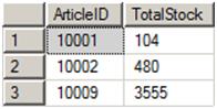
Figure 4: The #cteStockSum table
The second statement creates a table, #cteReverseInSum. The first interesting thing to notice is that Dave used an index hint to make sure that the special index he created was used. I’ll discuss more about index hints later in the article. The results of this statement is a list of all the IN and RET rows along with a backwards running total; in other words, how many items have been added to Stock, when looking at the back of the queue. Since we are concerned about the items left after all the processing is complete, we are concerned about the items added last.
The statement joins the Stock table to itself, using a correlated sub-query. A correlated sub-query cannot run independently because it references the outer query within the WHERE clause. In this case, after matching on ArticleID, all rows in the sub-query with a TranDate greater than or equal to the TranDate in the outer query are used to calculate the sum (this is referred to as a triangular join). The RollingStock column comes from the sub-query, and is a sum of the items added on the TranDate and later. The RollingStock values will be used to figure out which items are still in the queue at the end of the stock transactions. In other words, this query determines which of the transactions at the end of the queue actually added the items that are left once all transactions have completed. Figure 5 shows the reverse running totals for some of the rows for ArticleID 10009. The ThisStock column is the original number of items added during the transaction.
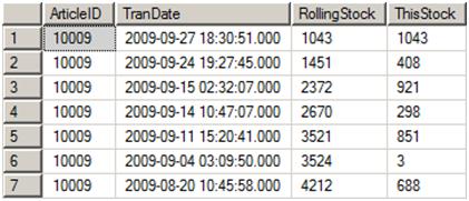
Figure 5: The #cteReverseInSum table rows for Article 10009
The next section of code creates the #cteWithLastTranDate table using the two temp tables created in the previous step. In the original code, the cteWithLastTranDate definition contained the two previously defined CTEs. Listing 10 shows the code. This statement also contains a correlated sub-query, but with a twist.
|
1 2 3 4 5 6 7 8 9 10 11 12 13 14 15 16 17 18 19 20 21 22 |
SELECT w.ArticleID , w.TotalStock , LastPartialStock.TranDate , LastPartialStock.StockToUse , LastPartialStock.RunningTotal , w.TotalStock - LastPartialStock.RunningTotal + LastPartialStock.StockToUse AS UseThisStock INTO #cteWithLastTranDate FROM #cteStockSum AS w CROSS APPLY ( SELECT TOP ( 1 ) z.TranDate , z.ThisStock AS StockToUse , z.RollingStock AS RunningTotal FROM #cteReverseInSum AS z WHERE z.ArticleID = w.ArticleID AND z.RollingStock >= w.TotalStock ORDER BY z.TranDate DESC ) AS LastPartialStock --Display the results SELECT * FROM #cteWithLastTranDate |
Listing 10: Creating #cteWithLastTranDate
The results of running Listing 10 can be seen in Figure 6. Once again, my code saves the results of David’s CTE into a temp table. The inner query in this section finds the first row from #cteReverseInSum that is at least the TotalStock value stored in the #cteStockSum table for each ArticleID. By using CROSS APPLY, this correlated sub-query looks like a derived table by appearing in the FROM clause and making more than one column available to the outer query. It is not a derived table, however, because a derived table does not reference the outer query. The CROSS APPLY operator allows the inner query to be applied once for each row of the outer query. You might wonder why the code doesn’t just join the two tables. In this case, we need to find one row from the inner query for every row of the outer query. If we use TOP(1) in a regular join, only one total row would be returned instead of one row for each ArticleID.
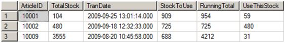
Figure 6: The #cteWithLastTranDate results
The SELECT list of the outer query contains the ArticleID and TotalStock from the #cteStockSum table. The next three columns (TranDate, StockToUse, and RunningTotal) are from the inner query based on #cteReverseInSum. Next in the list is a calculation, UseThisStock:
|
1 2 |
w.TotalStock - LastPartialStock.RunningTotal + LastPartialStock.StockToUse AS UseThisStock |
The calculation is used to determine how many items from the oldest row are required to cover the remaining items that will be needed. There are 3555 items of ArticleID 10009 left in stock. If you take a look at Figure 5 again, you will see that we have to go back to the seventh row containing 4212 in the RollingStock column to cover that amount. We need all the items in the first six rows and some of them from the seventh row. The most straightforward way to calculate this would be to subtract the RollingStock in the sixth row from the items needed, 3555 – 3524. Thirty-one items from the seventh row plus all the items added to stock from rows one through six remain in stock.
David figured out the difference between the covering row (row 7 in Figure 5) and the previous row is the number of items added. Now the calculation becomes 3555 – (4212 – 688), still equaling 31. Instead of looking back at row 6, he just subtracts the items added at row 7 from the running total. Now we have the number of items remaining from the earliest qualifying row without visiting the previous row to do the calculation. If you take a look at Figure 6 again, you will see a row for each ArticleID, showing the earliest transaction date required to cover the items left. The StockToUse column contains the number of items added at that transaction, and the UseThisStock column contains the number of items needed in addition to the transaction rows after this transaction.
The final statement provides the answer to the challenge. See Listing 11 for the code.
|
1 2 3 4 5 6 7 8 9 10 11 12 13 14 15 16 17 18 19 20 21 |
SELECT y.ArticleID , y.TotalStock AS CurrentItems , SUM(CASE WHEN e.TranDate = y.TranDate THEN y.UseThisStock ELSE e.Items END * Price.Price) AS CurrentValue FROM #cteWithLastTranDate AS y INNER JOIN dbo.Stock AS e WITH ( INDEX ( IX_Dave_Items ) ) ON e.ArticleID = y.ArticleID AND e.TranDate >= y.TranDate AND e.TranCode IN ('IN', 'RET' ) CROSS APPLY ( SELECT TOP ( 1 ) p.Price FROM dbo.Stock AS p WITH ( INDEX ( IX_Dave_Price ) ) WHERE p.ArticleID = e.ArticleID AND p.TranDate <= e.TranDate AND p.TranCode = 'IN' ORDER BY p.TranDate DESC ) AS Price GROUP BY y.ArticleID , y.TotalStock ORDER BY y.ArticleID |
Listing 11: The final answer
The first interesting feature of this statement is the query hints specifying which indexes the query should use. Even though this is called “hint”, the database engine is forced to follow whatever the hint specifies, even if the performance suffers. Caution is required when using hints, because the database engine usually does a better job optimizing the query without the hint. In this case, the indexes were strategically designed with this query in mind. Just to see what would happen, I removed the hints and found by viewing the execution plan that the database engine used the IX_Dave_Items index but not the IX_Dave_Price index. When comparing the execution times for each method against the original data, the original solution was just a couple of seconds faster with the hints.
At this point, just running the query in Listing 11 will give the answer. However, to take a closer look and figure out what is going on here, I removed the SUM function and the GROUP BY clause and expanded the column list (Listing 12).
|
1 2 3 4 5 6 7 8 9 10 11 12 13 14 15 16 17 18 19 20 21 22 23 24 25 26 |
SELECT y.ArticleID , y.TotalStock AS CurrentItems , e.TranDate , y.TranDate , y.UseThisStock , e.Items , Price.Price , CASE WHEN e.TranDate = y.TranDate THEN y.UseThisStock ELSE e.Items END * Price.Price AS CurrentValue FROM #cteWithLastTranDate AS y INNER JOIN dbo.Stock AS e WITH ( INDEX ( IX_Dave_Items ) ) ON e.ArticleID = y.ArticleID AND e.TranDate >= y.TranDate AND e.TranCode IN ('IN', 'RET' ) CROSS APPLY ( /* Find the Price of the item in */ SELECT TOP ( 1 ) p.Price FROM dbo.Stock AS p WITH ( INDEX ( IX_Dave_Price ) ) WHERE p.ArticleID = e.ArticleID AND p.TranDate <= e.TranDate AND p.TranCode = 'IN' ORDER BY p.TranDate DESC ) AS Price ORDER BY y.ArticleID |
Listing 12: The final query without aggregation
Figure 7 displays a sample of the results. This query joins the #cteWithLastTranDate table to the original Stock table. It also contains a correlated sub-query with CROSS APPLY, using Stock. The #cteWithLastTranDate table specifies the earliest row to use for each ItemID. By joining Stock, all the rows adding items to stock that are required for the solution are retrieved. Finally, the sub-query provides the prices. If the RET rows contained a price, this would not have been necessary. By using the sub-query, the query retrieves the price for IN rows and the previous price for RET rows.
Finally, the code contains a CASE statement in the SELECT list. If the TranDate in the row from Stock matches the TranDate in the earliest row – the one we where we need just some of the items – then use the calculated value. Otherwise, use the all the stock items for that row, the Items value.
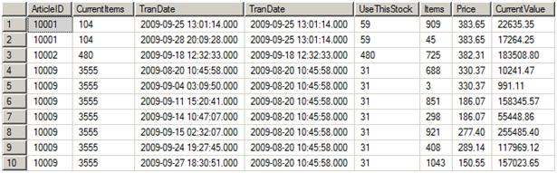
Figure 7: The unaggregated results
By reverting back to the query found in Listing 11, you will see the results of running David’s original script intact (Figure 8).
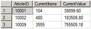
Figure 8: The final results for three ArticleIDs
Solution Highlights
The important thing to remember when solving this problem is that you need to focus on the items remaining in stock. You don’t have to calculate the current items and values for each transaction. Here are some other important things to learn from this solution:
- CTEs can be used to store intermediary results instead of temp tables
- CTEs can be based on other CTEs
- Use CROSS APPLY with a correlated sub-query when the sub-query must be applied once for each outer row and the normal rules for correlated sub-queries must be broken
- Use
TOP(1) and ORDER BY in a sub-query to return the first matching row Query hints can improve performance, but use caution since the database engine will follow the hint even if it hurts performance
Table 4 contains the results for each of the three methods.
|
Method |
Time |
|
Cursor |
40 minutes |
|
Solution with CTEs |
3 seconds |
|
Solution with temp tables using indexes |
18 seconds |
Table 4: The comparison
Conclusion
Sometimes the most seemingly straightforward problem is difficult to figure out if you haven’t seen it before. The description for this problem focuses on adding and removing items one transaction at a time. The solution, instead, requires that you focus on what is left after all processing is complete. Focusing on the information provided in the initial challenge will lead you down the wrong path; make sure you understand exactly what you need to do and do not waste time providing information outside the scope of the problem.

Load comments