The aim of this article is to enable you to interpret basic graphical execution plans, in other words, execution plans for simple SELECT, UPDATE, INSERT or DELETE queries, with only a few joins and no advanced functions or hints. In order to do this, we’ll cover the following graphical execution plan topics:

• Operators – introduced in the last article, now you’ll see more
• Joins – what’s a relational system without the joins between tables
• WHERE clause – you need to filter your data and it does affect the execution plans
• Aggregates – how grouping data changes execution plans
• Insert  Update and Delete execution plans

The Language of Graphical Execution Plans 

In some ways, learning how to read graphical execution plans is similar to learning a new language, except that the language is icon-based, and the number of words (icons) we have to learn is minimal. Each icon represents a specific operator within the execution plan. We will be using the terms ‘icon’ and ‘operator’ interchangeably in this article.

In the previous article, we only saw two operators (Select and Table Scan ). However, there are a total of 79 operators available. Fortunately for us, we don’t have to memorize all 79 of them before we can read a graphical execution plan. Most queries use only a small subset of the icons, and those are the ones we are going to focus on in this article. If you run across an icon not covered here, you can find out more information about it on Books Online:

Four distinct types of operator are displayed in a graphical execution plan:

• Logical and physical operators, also called iterators, are displayed as blue icons and represent query execution or Data Manipulation Language (DML) statements.
• Parallelism physical operators are also blue icons and are used to represent parallelism operations. In a sense, they are a subset of logical and physical operators, but are considered separate because they entail an entirely different level of execution plan analysis.
• Cursor operators have yellow icons and represent Transact-SQL cursor operations
• Language elements are green icons and represent Transact-SQL language elements, such as Assign, Declare, If, Select (Result), While, and so on.

In this article we’ll focus mostly on logical and physical operators, including the parallelism phys­ical operators. Books Online lists them in alphabetical order, but this is not the easiest way to learn them, so we will forgo being “alphabetically correct” here. Instead, we will focus on the most-used icons. Of course, what is considered most-used and least-used will vary from DBA to DBA, but the following are what I would consider the more common oper­ators, listed from left-to-right and top-to-bottom, roughly in the order of most common to least common:

Select (Result)	Sort	Clustered Index Seek	Clustered Index Scan	Non-clustered Index Scan
Non-clustered Index Seek	Table Scan	RID Lookup	Key Lookup	Hash Match
Nested Loops	Merge Join	Top	Compute Scalar	Constant Scan
Filter	Lazy Spool	Spool	Eager Spool	Stream Aggregate
Distribute Streams	Repartition Streams	Gather Streams	Bitmap	Split

Those picked out in bold are covered in this article. The rest will be covered in the book.

Operators have behavior that is worth understanding. Some operators – primarily sort, hash match (aggregate) and hash join  – require a variable amount of memory in order to execute. Because of this, a query with one of these operators may have to wait for available memory prior to execution, possibly adversely affecting performance. Most operators behave in one of two ways, non-blocking or blocking. A non-blocking operator creates output data at the same time as it receives the input. A blocking operator has to get all the data prior to producing its output. A blocking operator might contribute to concurrency problems, hurting performance.

Some Single table Queries

Let’s start by looking at some very simple plans, based on single table queries.

Clustered Index Scan   

Consider the following simple (but inefficient!) query against the Person.Contact table in the AdventureWorks database:

Following is the actual execution plan:

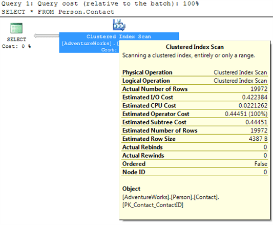
Figure 1

We can see that a clustered index scan operation is performed to retrieve the required data. If you place the mouse pointer over the Clustered Index Scan  icon, to bring up the ToolTip window, you will see that the clustered index used was PK_Contact_ContactID and that the estimated number of rows involved in the operation was 19972.

Indexes in SQL Server are stored in a B-tree (a series of nodes that point to a parent). A clustered index not only stores the key structure, like a regular index, but also sorts and stores the data, which is the main reason why there can be only one clustered index per table.

As such, a clustered index scan is almost the same in concept as a table scan. The entire index, or a large percentage of it, is being traversed, row-by-row, in order to identify the data needed by the query.

An index scan often occurs, as in this case, when an index exists but the optimizer determines that so many rows need to be returned that it is quicker to simply scan all the values in the index rather than use the keys provided by that index.

An obvious question to ask if you see an index scan in your execution plan is whether you are returning more rows than is necessary. If the number of rows returned is higher than you expect, that’s a strong indication that you need to fine-tune the WHERE clause of your query so that only those rows that are actually needed are returned. Returning unnecessary rows wastes SQL Server resources and hurts overall performance.

Clustered Index Seek   

We can easily make the previous query more efficient by adding a WHERE clause:

The plan now looks as shown in figure 2:

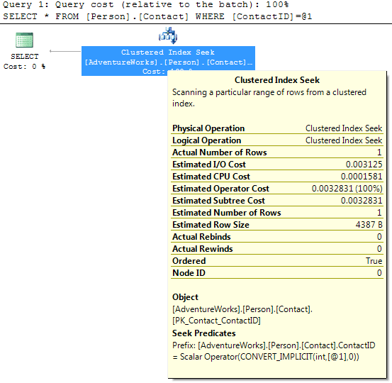
Figure 2

Index seeks are completely different from scans, where the engine walks through the rows to find what it needs. An index seek, clustered or not, occurs when the optimizer is able to locate an index that it can use to retrieve the required records. Therefore, it tells the storage engine to look up the values based on the keys of the given index. Indexes in SQL Server are stored in a B-tree (a series of nodes that point to a parent). A clustered index stores not just the key structure, like a regular index, but also sorts and stores the data, which is the main reason why there can be only one clustered index per table.

When an index is used in a seek operation, the key values are used to quickly identify the row, or rows, of data needed. This is similar to looking up a word in the index of a book to get the correct page number. The added value of the clustered index seek is that, not only is the index seek an inexpensive operation as compared to an index scan, but no extra steps are required to get the data because it is stored in the index.

In the above example, we have a Clustered Index Seek operation carried out against the Person.Contact table, specifically on the PK_Contact_ContactId, which is happens to be both the primary key and the clustered index for this table.

Note on the ToolTips window for the Clustered Index Seek that the Ordered property is now true, indicating that the data was ordered by the optimizer.

Non-clustered Index Seek   

Let’s run a slightly different query against the Person.Contact table; one that uses a non-clustered index:

We get a non-clustered index seek. Notice in the ToolTip shown in figure 3 that the non-clustered index, IX_Contact_EmailAddress has been used.

NOTE: The non-clustered Index Seek icon is misnamed and called an Index Seek in the execution plan below. Apparently, this was a mistake by Microsoft and hopefully will be fixed at some point. No big deal, but something for you to be aware of.

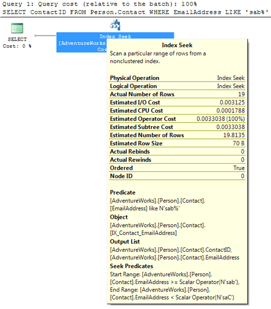
Figure 3

Like a clustered index seek, a non-clustered index seek uses an index to look up the rows to be returned directly. Unlike a clustered index seek, a non-clustered index seek has to use a non-clustered index to perform the operation. Depending on the query and index, the query optimizer might be able to find all the data in the non-clustered index, or it might have to look up the data in the clustered index, slightly hurting performance due to the additional I/O required to perform the extra lookups – more on this in the next section.

Key LookUp  

Let’s take our query from the previous sections and alter it so that it returns just a few more columns:

You should see a plan like that shown in figure 4:

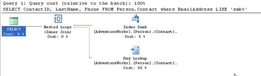
Figure 4

Finally, we get to see a plan that involves more than a single operation! Reading the plan from right-to-left and top-to-bottom, the first operation we see is an Index Seek against the IX_Contact_EmailAddress index. This is a non-unique, non-clustered index and, in the case of this query, it is non-covering. A non-covering index is an index that does not contain all of the columns that need to be returned by a query, forcing the query optimizer to not only read the index, but to also read the clustered index to gather all the data it needs so it can be returned.

We can see this in the ToolTips window from the Output List for the Index Seek, in figure 5, which shows the EmailAddress and ContactID columns.

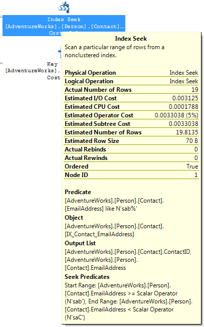
Figure 5

The key values are then used in a Key Lookup on the PK_Contact_ContactID clustered index to find the corresponding rows, with the output list being the LastName and Phone columns, as shown in figure 6.

 

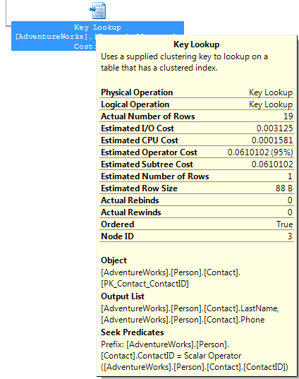
Figure 6

A Key Lookup is a bookmark lookup on a table with a clustered index. (Pre-SP2, this operation would have been represented with a Clustered Index scan, with a LookUp value of True) .

A Key Lookup essentially means that the optimizer cannot retrieve the rows in a single operation, and has to use a clustered key (or a row ID) to return the corresponding rows from a clustered index (or from the table itself).

The presence of a Key Lookup is an indication that query performance might benefit from the presence of a covering or included index. Both a covering or included index include all of the columns that need to be returned by a query, so all the columns of each row are found in the index, and a Key Lookup does not have to occur in order to get all the columns that need to be returned.

A Key LookUp is always accompanied by the Nested Loop join operation that combines the results of the two operations.

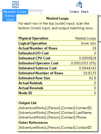
Figure 7

Typically, a Nested Loops join is a standard type of join and by itself does not indicate any performance issues. In this case, because a Key Lookup operation is required, the Nested Loops join is needed to combine the rows of the Index Seek and Key Lookup. If the Key Lookup was not needed (because a covering index was available), then the Nested Loops operator would not be needed and would not appear in the graphical execution plan.

Table Scan 

This operator is fairly self-explanatory and is one we previously encountered in Article 1. It indicates that the required rows were returned by scanning the table, one row after another. You can see a table scan operation by executing the following query:

SELECT  *

FROM    [dbo].[DatabaseLog]

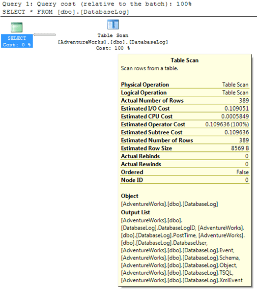
Figure 8

A table scan can occur for several reasons, but it’s often because there are no useful indexes on the table, and the query optimizer has to search through every row in order to identify the rows to return. Another common reason why a table scan may occur is when all the rows of a table are returned, as is the case in this example. When all (or the majority) of the rows of a table are returned then, whether an index exists or not, it is often faster for the query optimizer to scan through each row and return them than look up each row in an index. And last, sometimes the query optimizer determines that it is faster to scan each row than it is to use an index to return the rows. This commonly occurs in tables with few rows.

Assuming that the number of rows in a table is relatively small, table scans are generally not a problem. On the other hand, if the table is large and many rows are returned, then you might want to investigate ways to rewrite the query to return fewer rows, or add an appropriate index to speed performance.

RID LookUp 

If we specifically filter the results of our previous DatabaseLog query using the primary key column, we see a different plan that uses a combination of an Index Seek   and a RID LookUp .

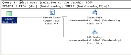
Figure 9

To return the results for this query, the query optimizer first performs an Index Seek on the primary key. While this index is useful in identifying the rows that meet the WHERE clause criteria, all the required data columns are not present in the index. How do we know this?

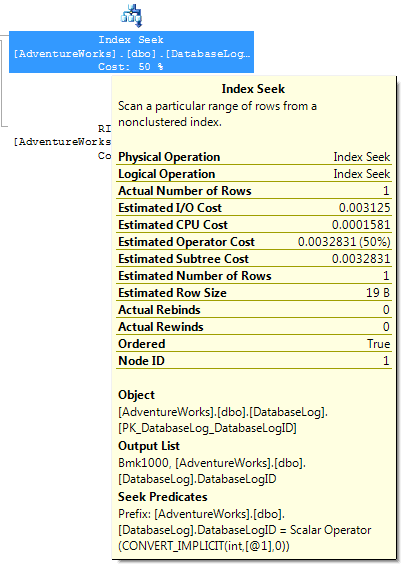
Figure 10

If you look at the ToolTip above for the Index Seek, we see “Bmk1000″ is in the Output list. This”Bmk1000” is telling us that this Index Seek is actually part of a query plan that has a bookmark lookup.

Next, the query optimizer performs a RID LookUp, which is a type of bookmark lookup that occurs on a heaptable (a table that doesn’t have a clustered index), and uses a row identifier to find the rows to return. In other words, since the table doesn’t have a clustered index (that includes all the rows), it must use a row identifier that links the index to the heap. This adds additional disk I/O because two different operations have to be performed instead of a single operation, which are then combined with a Nested Loops operation.

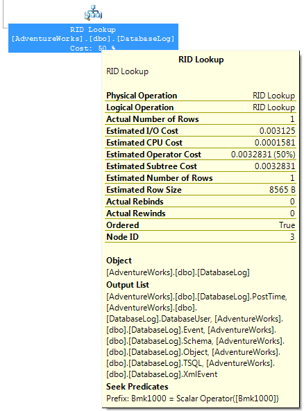
Figure 11

In the above ToolTip for the RID Lookup, notice that “Bmk1000” is used again, but this time in the Seek Predicates section. This is telling us that a bookmark lookup (specifically a RID Lookup in our case) was used as part of the query plan. In this particular case, only one row had to be looked up, which isn’t a big deal from a performance perspective. But if a RID Lookup returns many rows, you should consider taking a close look at the query to see how you can make it perform better by using less disk I/O – perhaps by rewriting the query, by adding a clustered index, or by using a covering or included index.

Table Joins 

Up to now, we have worked with single tables. Let’s spice things up a bit and introduce joins into our query. The following query retrieves employee information, concatenating the FirstName and LastName columns in order to return the information in a more pleasing manner.

The execution plan for this query is shown in figure 12.

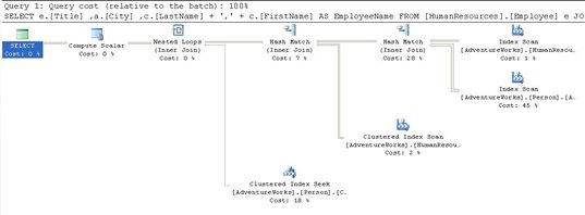
Figure 12

With this query there are multiple processing steps occurring, with varying costs to the processor. The cost accumulates as you move thorough the execution tree from right to left.

From the relative cost displayed below each operator icon, we can identify the three most costly operations in the plan, in descending order:

1.  The Index Scan against the Person.Address table (45%)

2. The Hash Match join operation between the HumanResources.EmployeeAddress and Person.Address (28%)

3. The Clustered Index Seek on the Person.Contact table (18%)

Let’s consider each of the operators we see in this plan.

Starting on the right of Figure 12 above, the first thing we see is an Index Scan against the HumanResources.EmployeeAddress table, and directly below this is another index scan against the Person.Address table. The latter was the most expensive operation in the plan, so let’s investigate further. By bringing up the ToolTip, shown in Figure 13, we can see that the scan was against the index IX_Address_AddressLine_­AddressLine2_­City_­StateProvinceId_­PostalCode and that the storage engine had to walk through 19,614 rows to arrive at the data that we needed.

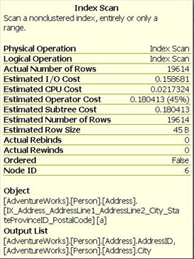
Figure 13

The query optimizer needed to get at the AddressId and the City columns, as shown by the output list. The optimizer calculated, based on the selectivity of the indexes and columns in the table, that the best way to arrive at that data was to walk though the index. Walking through those 19,614 rows took 45% of the total query cost or an estimated operator cost of 0.180413. The estimated operator cost is the cost to the query optimizer for executing this specific operation, which is an internally calculated number used by the query optimizer to evaluate the relative costs of specific operations. The lower this number, the more efficient the operation.

Hash Match   (Join) 

Continuing with the above example, the output of the two index scans is combined through a Hash Match  join  , the second most expensive operation of this execution plan. The ToolTip for this operator is shown in Figure 14:

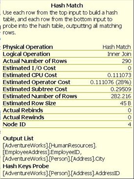
Figure 14

Before we can talk about what a Hash Match join is, we need to understand two new concepts: hashing and hash table . Hashing is a programmatic technique where data is converted into a symbolic form that makes it easier to be searched for quickly. For example, a row of data in a table can be programmatically converted into a unique value that represents the contents of the row. In many ways it is like taking a row of data and encrypting it. Like encryption, a hashed value can be converted back to the original data. Hashing is often used within SQL Server to convert data into a form that is more efficient to work with, or in this case, to make searching more efficient.

A hash table, on the other hand, is a data structure that divides all of the elements into equal-sized categories, or buckets, to allow quick access to the elements. The hashing function determines which bucket an element goes into. For example, you can take a row from a table, hash it into a hash value, then store the hash value into a hash table.

Now that we understand these terms, a Hash Match  join occurs when SQL Server joins two tables by hashing the rows from the smaller of the two tables to be joined, and then inserting them into a hash table, then processing the larger table one row at a time against the smaller hashed table, looking for  matches where rows need to be joined. Because the smaller of the tables provides the values in the hash table, the table size is kept at a minimum, and because hashed values instead of real values are used, comparisons can be made very quickly. As long as the table that is hashed is relatively small, this can be a quick process. On the other hand, if both tables are very large, a Hash Match join can be very inefficient as compared to other types of joins.

In this example, the data from HumanResources.EmployeeAddress.AddressId is matched with Person.Address table.

Hash Match joins are often very efficient with large data sets, especially if one of the tables is substantially smaller than the other. Hash Match joins also work well for tables that are not sorted on join columns, and they can be efficient in cases where there are no useable indexes. On the other hand, a Hash Match join might indicate that a more efficient join method (Nested Loops or Merge) could be used. For example, seeing a Hash Match join in an execution plan sometimes indicates:

• a missing or incorrect index

• a missing WHERE clause

• a WHERE clause with a calculation or conversion that makes it non-sargeable (a commonly used term meaning that the search argument, “sarg” can’t be used). This means it won’t use an existing index.

While a Hash Match join may be the most efficient way for the query optimizer to join two tables, it does not mean there are not more efficient ways to join two tables, such as adding appropriate indexes to the joined tables, reducing the amount of data returned by adding a more restrictive WHERE clause, or by making the WHERE clause sargeble. In other words, a seeing a Hash Match join should be a cue for you to investigate if the join operation can be improved or not. If it can be improved, then great. If not, then there is nothing else to do, as the Hash Match join might be the best overall way to perform the join.

Worth noting in this example is the slight discrepancy between the estimated number of rows returned, 282.216 (proving this is a calculation since you can’t possibly return .216 rows), and the actual number of rows, 290. A difference this small is not worth worrying about, but a larger discrepancy indicates that your statistics are out of date and need to be updated. A large difference can lead to differences in the Estimated and Actual plans.

The query proceeds from here with another index scan against the HumanResources­.Employee table and another Hash Match between the results of the first Hash Match and the index scan.

Clustered Index Seek   

After the Hash Match   Join, we see a Clustered Index Seek    operation carried out against the Person.Contact table, specifically on the PK_Contact_ContactId, which is both the primary key and clustered index for this table. This is the third most-expensive operation in the plan. The ToolTip is shown in Figure 15.

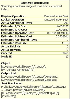
Figure15

Note from the Seek Predicates  section in figure 15 above, that the operation was joining directly between the ContactId column in the HumanResources.Employee table and the Person.Contact table.

Nested Loops Join  

Following the clustered index seek, the data accumulated by the other operations are joined with the data collected from the seek, through a Nested Loops  Join    , as shown in Figure 16.

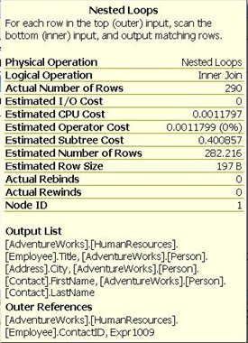
Figure 16

The nested loops join is also called a nested iteration. This operation takes the input from two sets of data and joins them by scanning the outer data set (the bottom operator in a graphical execution plan) once for each row in the inner set. The number of rows in each of the two data sets was small, making this a very efficient operation. As long as the inner data set is small and the outer data set, small or not, is indexed, this becomes an extremely efficient join mechanism. Unless you have very large data sets, this is the type of join that you most want to see in an execution plan.

Compute Scalar 

Finally, in the execution plan shown in figure 12, right before the Select operation, we have a Compute Scalar operation. The Tooltip for this operator is shown in Figure 19.

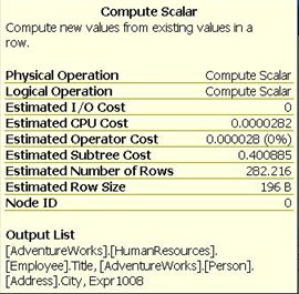
Figure 19

This is simply a representation of an operation to produce a scalar, a single defined value, usually from a calculation – in this case, the alias EmployeeName which combines the columns Contact.LastName and Contact.FirstName with a comma in between them. While this was not a zero-cost operation, 0.0000282, it’s so trivial in the context of the query as to be essentially free of cost.

Merge Join 

Besides the Hash and Nested Loops Join , the query optimizer can also perform a Merge Join . To seen an example of a Merge Join, we can run the following code in the AdventureWorks database:

SELECT  c.CustomerID
FROM    Sales.SalesOrderDetail od
        JOIN Sales.SalesOrderHeader oh
            ON od.SalesOrderID = oh.SalesOrderID
        JOIN Sales.Customer c    
       ON oh.CustomerID = c.CustomerID

The above query produces an execution plan that looks as shown in figure 17.

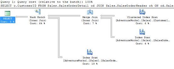
Figure 17

According to the execution plan, the query optimizer performs a Clustered Index Scan on the Customer table and a non-clustered Index Scan   on the SalesOrderHeader table. Since a WHERE clause was not specified in the query, a scan was performed on each table to return all the rows in each table.

Next, all the rows from both the Customer and SalesOrderHeader tables are joined using the Merge Join  operator. A Merge Join occurs on tables where the join columns are presorted. For example, in the ToolTip window for the Merge Join, shown in figure 18, we see that the join columns are Sales and CustomerID. In this case, the data in the join columns are presorted in order. A Merge Join is an efficient way to join two tables, when the join columns are presorted but if the join columns are not presorted, the query optimizer has the option of a) sorting the join columns first, then performing a Merge Join, or b) performing a less efficient Hash Join. The query optimizer considers all the options and generally chooses the execution plan that uses the least resources.

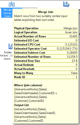
Figure 18

Once the Merge Join has joined two of the tables, the third table is joined to the first two using a Hash Match Join, which was discussed earlier. And finally, the joined rows are returned.

The key to performance of a Merge Join is that the joined columns are already presorted. If they are not, and the query optimizer chooses to sort the data before it performs a Merge Join, and this might be an indication that a Merge Join is not an ideal way to join the tables, or it might indicate that you need to consider some different indexes.

Adding a WHERE Clause

Only infrequently will queries run without some sort of conditional statements to limit the results set:; in other words, a WHERE clause. We’ll investigate two multi-table, conditional queries using graphical execution plans.

Run the following query against AdventureWorks, and look at the actual execution plan. This query is the same as the one we saw at the start of the Table Joins  section, but now has a WHERE clause.

Figure 20 shows the actual execution plan for this query:

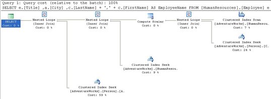
Figure 20

Starting from the right, we see that the optimizer has used the criteria from the WHERE clause to do a clustered index scan, using the primary key. The WHERE clause limited the number of rows to 22, which you can see by hovering your mouse pointer over the arrow coming out of the Clustered Index Scan    operator (see figure 21).

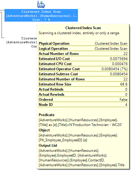
Figure 21

The optimizer, using the available statistics, was able to determine this up front, as we see by comparing the estimated and actual rows returned in the ToolTip.

Working with a smaller data set and a good index on the Person.Contact table, as compared to the previous query, the optimizer was able to use the more efficient Nested Loop    Join    . Since the optimizer changed where that table was joined, it also moved the scalar calculation right next to the join. Since it’s still only 22 rows coming out of the scalar operation, a clustered index seek and another nested loop were used to join the data from the HumanResources.EmployeeAddress table. This then leads to a final clustered index seek and the final nested loop. All these more efficient joins are possible because we reduced the initial data set with the WHERE clause, as compared to the previous query which did not have a WHERE clause.

Frequently, developers who are not too comfortable with T-SQL will suggest that the “easiest” way to do things is to simply return all the rows to the application, either without joining the data between tables, or even without adding the WHERE clause. This was a very simple query with only a small set of data, but you can use this as an example, when confronted with this sort of argument. The final subtree cost for the optimizer for this query, when we used a WHERE clause, was 0.112425. Compare that to the 0.400885 of the previous query. That’s four times faster even on this small, simple query. Just imagine what it might be like when the data set gets bigger and the query becomes more complicated.

Execution Plans with GROUP BY and ORDER BY

When other basic clauses are added to a query, different operators are displayed in the execution plans.

Sort 

  

Take a simple select with an ORDER BY clause as an example:

The execution plan  is shown in figure 22.

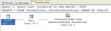
Figure 22

The Clustered Index Scan    operator outputs into the Sort   operator. Compared to many of the execution plan icons, the Sort operator is very straightforward. It literally is used to show when the query optimizer is sorting data within the execution plan. If an ORDER BY clause does not specify order, the default order is ascending, as you will see from the ToolTip for the Sort icon (see figure 23 below).

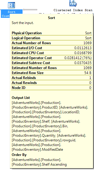
Figure 23

If you pull up the ToolTip window for the Sort icon (see figure 24), you’ll see that the Sort operator is being passed 1069 rows. The Sort operator takes these 1069 rows from the Clustered Index Scan , sorts them, and then passes the 1069 rows back in sorted order.

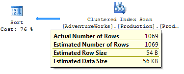
Figure 24

The most interesting point to note is that the Sort operation is 76% of the cost of the query. There is no index on this column, so the Sort operation is done within the query execution.

As a rule-of-thumb, I would say that when sorting takes more than 50% of a query’s total execution time, then you need to carefully review it to ensure that it is optimized. In our case the reason why we are breaking this rule is fairly straightforward: we are missing a WHERE clause. Most likely, this query is returning more rows to be sorted than needs to be returned. However, even if a WHERE clause exists, you need to ensure that it limits the amount of rows to only the required number of rows to be sorted, not rows that will never be used.

Other things to consider are:

• Is the sort really necessary? If not, remove it to reduce overhead.
• Is it possible to have the data presorted so it doesn’t have to be sorted? For example, can a clustered index be used that already sorts the data in the proper order? This is not always possible, but if it is, you will save sorting overhead if you create the appropriate clustered index.
• If an execution plan has multiple Sort   operators, review the query to see if they are all necessary, or if the code can be rewritten so that fewer sorts are needed to accomplish the goal of the query.

If we change the query to the following:

We get the execution plan shown in figure 25:

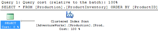
 Figure 25

Although this query is almost identical to the previous query, and it includes an ORDER BY clause, we don’t see a sort operator in the execution plan. This is because the column we are sorting by has changed, and this new column has a clustered index on it, which means that the returned data does not have to be sorted again, as it is already sorted as a byproduct of it being the clustered index. The query optimizer is smart enough to recognize that the data is already ordered, and does not have to order it again. If you have no choice but to sort a lot of data, you should consider using the SQL Server 2005 Profiler to see if any Sort Warnings are generated. To boost performance, SQL Server 2005 attempts to perform sorting in memory instead of disk. Sorting in RAM is much faster than sorting on disk. But if the sort operation is large, SQL Server may not be able to sort the data in memory, instead, having to write data to the tempdb database. Whenever this occurs, SQL Server generates a Sort Warning event, which can be captured by Profiler. If you see that your server is performing a lot of sorts, and many Sort Warnings are generated, then you may need to add more RAM to your server, or to speed up tempdb access.

Hash Match (Aggregate)

Earlier in this article, we took a look at the Hatch Match operator for joins. This same Hatch Match operator also can occur when aggregations occur within a query. Let’s consider a simple aggregate query against a single table using the COUNT operator:

The actual execution plan is shown below.

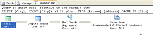
Figure 26

The query execution begins with an Index Scan, because all of the rows are returned for the query. There is no WHERE clause to filter the rows. These rows then need to be aggregated in order to perform the requested COUNT aggregate operation. In order for the query optimizer to count each row for each separate city, it must perform a Hatch Match operation. Notice that underneath Hatch Match in the execution plan that the word “aggregate” is put between parentheses. This is to distinguish it from a Hatch Match operation for a join. As with a Hatch Match with a join, a Hatch Match with an aggregate causes SQL Server to create a temporary hash table in memory in order to count the number of rows that match the GROUP BY column, which in this case is “City.” Once the results are aggregated, then the results are passed back to us.

Quite often, aggregations with queries can be expensive operations. About the only way to “speed” the performance of an aggregation via code is to ensure that you have a restrictive WHERE clause to limit the number of rows that need to be aggregated, thus reducing the amount of aggregation that needs to be done.

Filter

If we add a simple HAVING clause to our previous query, our execution plan gets more complex

The execution plan now looks as shown in figure 27:

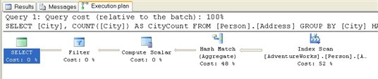
Figure 27

By adding the HAVING clause, the Filter operator has been added to the execution plan. We see that the Filter operator is applied to limit the output to those values of the column, City, that are greater than 1. One useful bit of knowledge to take away from this plan is that the HAVING clause is not applied until all the aggregation of the data is complete. We can see this by noting that the actual number of rows in the Hash Match  operator is 575 and in the Filter operator it’s 348.

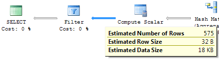
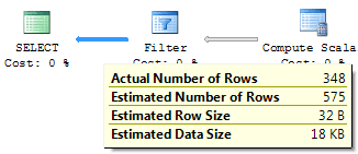
Figure 28

While adding a HAVING clause reduces the amount of data returned, it actually adds to the resources needed to produce the query results, because the HAVING clause does not come into play until after the aggregation. This hurts performance. As with the previous example, if you want to speed the performance of a query with aggregations, the only way to do so in code is to add a WHERE clause to the query to limit the number of rows that need to be selected and aggregated.

Rebinds and Rewinds Explained 

While examining the ToolTips for physical operators, throughout this article, you will have seen these terms several times:

• Actual Rebinds or Estimated Rebinds

• Actual Rewind or Estimated Rewinds

Most of the time in this article, the value for both the rebinds and rewinds has been zero, but for the Sort   operator example, a little earlier, we saw that there was one actual rebind and zero actual rewinds.

In order to understand what these values mean, we need some background. Whenever a physical operator, such as the SORT operator in an execution plan occurs, three things happen.

• First, the physical operator is initialized and any required data structures are set up. This is called the Init() method. In all cases this happens once for an operator, although it is possible to happen many times.
• Second, the physical operator gets (or receives) the rows of data that it is to act on. This is called the GetNext() method. Depending on the type of operator, it may receive none, or many GetNext() calls.
• Third, once the operator is done performing its function, it needs to clean itself up and shut itself down. This is called the Close() method. A physical operator only ever receives a single Close() call.

A rebind or rewind is a count of the number of times the Init() method is called by an operator. A rebind and a rewind both count the number of times the Init() method is called, but do so under different circumstances.

A rebind count occurs when one or more of the correlated parameters of a join change and the inner side must be reevaluated. A rewind count occurs when none of the correlated parameters change and the prior inner result set may be reused. Whenever either of these circumstances occur, a rebind or rewind occurs, and increases their count.

Given the above information, you would expect to see a value of one or higher for the rebind or rewind in every ToolTips or Properties screen for a physical operator. But you don’t. What is odd is that the rebind and rewind count values are only populated when particular physical operators occur, and are not populated when other physical operators occur. For example, if any of the following six operators occur, the rebind and rewind counts are populated:

• Nonclustered Index Spool 
• Remote Query
• Row Count Spool
• Sort 
• Table Spool 
• Table-Valued Function

If the following operators occur, the rebind and rewind counts will only be populated when the StartupExpression  for the physical operation is set to TRUE, which can vary depending on how the query optimizer evaluates the query. This is set by Microsoft in code and is something we have no control over.

• Assert 
• Filter

And for all other physical operators, they are not populated. In these cases, the counts for rebind zero count doeot mean that zero rebinds or rewinds occurred, just that these values were not populated. As you can imagine, this can get a little confusing. This also explains why most of the time you see zero values for rebind and rewind.

So, what does it mean when you see a value for either rebind or rewind for the eight operators where rebind and rewind may be populated?

If you see an operator where rebind equals one and rewinds equals zero, this means that an Init() method was called one time on a physical operator that is NOT on the inner side of a loop join. If the physical operator is ON the inner side of a loop join used by an operator, then the sum of the rebinds and rewinds will equal the number of rows process on the outer side of a join used by the operator

So how is this helpful to the DBA? Generally speaking, it is ideal if the rebind and rewind counts are as low as possible, as higher counts indicate more disk I/O. If the counts are high, it might indicate that a particular operator is working harder than it needs to, hurting server performance. If this is the case, it might be possible to rewrite the query, or modify current indexing, to use a different query plan that uses fewer rebinds and rewinds, reducing I/O and boosting performance.

Insert  Update and Delete Execution Plans

Execution plans are generated for all queries against the database in order for the engine to figure out how best to undertake the request you’ve submitted. While the previous examples have been for SELECT queries, in this section we will take a look at the execution plans of INSERT, UPDATE, and DELETE queries.

Insert Statements 

Here is a very simple INSERT statement:

This statement generates this rather interesting estimated plan (so that I don’t actually affect the data within the system), shown in Figure 29.

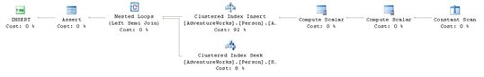
Figure 29

The execution plan starts off, reading right to left, with an operator that is new to us: Constant Scan . This operator introduces a constant number of rows into a query. In our case, it’s building a row in order for the next two operators to have a place to add their output. The first of these is a Compute Scalar  operator to call a function called getidentity. This is the moment within the query plan when an identity value is generated for the data to follow. Note that this is the first thing done within the plan, which helps explain why, when an insert fails, you get a gap in the identity values for a table.

Another scalar operation occurs which outputs a series of placeholders for the rest of the data and creates the new uniqueidentifier   value, and the date and time from the GETDATE function. All of this is passed to the Clustered Index Insert    operator, where the majority of the cost of this plan is realized. Note the output value from the INSERT statement, the Person.Address.StateProvinceId. This is passed to the next operator, the Nested Loop    join, which also gets input from the Clustered Index Seek    against the Person.StateProvince table. In other words, we had a read during the INSERT to check for referential integrity on the foreign key of StateProvinceId. The join then outputs a new expression which is tested by the next operator, Assert  . An Assert verifies that a particular condition exists. This one checks that the value of Expr1014 equals zero. Or, in other words, that the data that was attempted to be inserted into the Person.Address.StateProvinceId field matched a piece of data in the Person.StateProvince table; this was the referential check.

Update Statements 

Consider the following update statement:

The estimated execution plan is shown below:

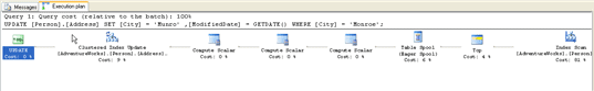
Figure 30

Let’s begin reading this execution plan, from right to left. The first operator is a non-clustered Index Scan, which retrieves all of the necessary rows from a non-clustered index, scanning through them, one row at a time. This is not particular efficient and should be a flag to you that perhaps the table needs better indexes to speed performance. The purpose of this operator is to identify all the rows WHERE [City] = ‘Monroe’, and then send them to the next operator.

The next operator is TOP. In an UPDATE execution plan, it is used to enforce row count limits, if there are any. In this case, no limits have been enforced because the TOP clause was not used in the UPDATE query.

Note: If the TOP operator is found in a SELECT statement, not an UPDATE statement, it indicates that a specified number, or percent, of rows have been returned, based on the TOP command used in the SELECT statement.

The next operator is an Eager Spool  (a form of a Table Spool  ). This obscure sounding operator essentially takes each of the rows to be updated and stores them in a hidden temporary object stored in the tempdb database. Later in the execution plan, if the operator is rewound (say due to the use of a Nested Loops operator in the execution plan) and no rebinding is required, the spooled data can be reused instead of having to rescan the data again (which means the non-clustered Index Scan has to be repeated, which would be an expensive option). In this particular query, no rewind operation was required.

The next three operators are all Compute Scalar operators, which we have seen before. In this case, they are used to evaluate expressions and to produce a computed scalar value, such as the GETDATE() function used in the query.

Now we get to the core of the UPDATE statement, the Clustered Index Update operator. In this case, the values being updated are part of a clustered index. So this operator identifies the rows to be updated, and updates them.

And last of all, we see the generic T-SQL Language Element Catchall operator, which tells us that an UPDATE operation has been completed.

From a performance perspective, one of the things to watch for is how the rows to be updated are retrieved. In this example, an non-clustered Index Scan was performed, which is not very efficient. Ideally, a clustered or non-clustered index seek would be preferred from a performance standpoint, as either one of them would use less I/O to perform the requested UPDATE.

Delete Statements 

What kind of execution plan is created with a DELETE statement? For example, let’s run the following code and check out the execution plan.

Figure 31 shows the estimated execution plan:

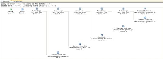
Figure 31

I know this is a bit difficult to read. I just wanted to show how big a plan is necessary to delete data within a relational database. Remember, removing a row, or rows, is not an event isolated to the table in question. Any tables related to the primary key of the table where we are removing data will need to be checked, to see if removing this piece of data affects their integrity. To a large degree, this plan looks more like a SELECT statement than a DELETE statement.

Starting on the right, and reading top to bottom, we immediately get a Clustered Index Delete operator. There are a couple of interesting points in this operation. The fact that the delete occurs at the very beginning of the process is good to know. The second interesting fact is that the Seek Predicate on this Clustered Index Seek    To Delete  operation was:

Prefix: [AdventureWorks].[Person].[Address].AddressID = Scalar Operator­(CONVERT_IMPLICIT(int,[@1],0)).

This means that a parameter, @1, was used to look up the AddressId. If you’ll notice in the code, we didn’t use a parameter, but rather used a constant value, 52. Where did the parameter come from? This is an indication of the query engine generating a reusable query plan, as per the rules of simple parameterization.

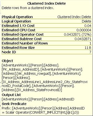
Figure 32

After the delete, a series of Index and Clustered Index Seek  s and Scans are combined through a series of Nested Loop Join operators. These are specifically Left Semi Joins. These operators return a value if the join predicate between the two tables in question matches or if there is no join predicate supplied. Each one returns a value. Finally, at the last step, an Assertoperator, the values returned from each Join, all the tables related to the table from which we’re attempting to delete data, are checked to see if referential data exists. If there is none, the delete is completed. If they do return a value, an error would be generated, and the DELETE operation aborted.

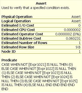
Figure 33

Summary

This article represents a major step in learning how to read graphical execution plans. However, as we discussed at the beginning of this article, we only focused on the most common type of operators and we only looked at simple queries. So if you decide to analyze a 200-line query and get a graphical execution plan that is just about as long, don’t expect to be able to analyze it immediately. Learning how to read and analyze execution plans takes time and effort. But once you gain some experience, you will find that it becomes easier and easier to read and analyze, even for the most complex of execution plans.